nLab topology
Context
Topology
topology (point-set topology, point-free topology)
see also differential topology, algebraic topology, functional analysis and topological homotopy theory
Basic concepts
-
fiber space, space attachment
Extra stuff, structure, properties
-
Kolmogorov space, Hausdorff space, regular space, normal space
-
sequentially compact, countably compact, locally compact, sigma-compact, paracompact, countably paracompact, strongly compact
Examples
Basic statements
-
closed subspaces of compact Hausdorff spaces are equivalently compact subspaces
-
open subspaces of compact Hausdorff spaces are locally compact
-
compact spaces equivalently have converging subnet of every net
-
continuous metric space valued function on compact metric space is uniformly continuous
-
paracompact Hausdorff spaces equivalently admit subordinate partitions of unity
-
injective proper maps to locally compact spaces are equivalently the closed embeddings
-
locally compact and second-countable spaces are sigma-compact
Theorems
Analysis Theorems
This page is about topology as a field of mathematics. For topology as a structure on a set, see topological space.
Parts of this page exists also in a German language version, see at Topologie.
Contents
- Idea
- Introduction
- Continuity
- Topological spaces
- Homeomorphism
- Homotopy
- Connected components
- Fundamental group
- Covering spaces
- Basic facts
- Central theorems
- Related entries
- Topological spaces
- Manifolds and generalizations
- Algebraic topology and homotopy theory
- Sheaves, stacks, cohomology
- Non-commutative topology
- Topological physics
- Computational Topology
- References
I believe that we lack another analysis properly geometric or linear which expresses location directly as algebra expresses magnitude.
G. W. Leibniz (letter to Huygens 1679, according to Bredon 93, p. 430)
Idea
Topology is one of the basic fields of mathematics. The term is also used for a particular structure in a topological space; see topological structure for that.
The subject of topology deals with the expressions of continuity and boundary, and studying the geometric properties of (originally: metric) spaces and relations of subspaces, which do not change under continuous deformations, regardless to other (such as in their metric properties).
Topology as a structure enables one to model continuity and convergence locally. More recently, in metric spaces, topologists and geometric group theorists started looking at asymptotic properties at large, which are in some sense dual to the standard topological structure and are usually referred to as coarse topology.
There are many cousins of the concept of topological spaces, e.g. sites, locales, topoi, higher topoi, uniformity spaces and so on, which specialize or generalize some aspect or structure usually found in Top.
One of the tools of topology, homotopy theory, has long since crossed the boundaries of topology and applies to many other areas, thanks to many examples and motivations as well as of abstract categorical frameworks for homotopy like Quillen model categories, Brown’s categories of fibrant objects and so on.
Introduction
The following gives a quick introduction to some of the core concepts and tools of topology:
A detailed introduction is going to be at Introduction to Topology.
Continuity
The key idea of topology is to study spaces with “continuous maps” between them. The concept of continuity was made precise first in analysis, in terms of epsilontic analysis of open balls, recalled as def. below. Then it was realized that this has a more elegant formulation in terms of the more general concept of open sets, this is prop. below. Adopting the latter as the definition leads to the concept of topological spaces, def. below.
First recall the basic concepts from analysis:
Definition
(metric space)
A metric space is
-
a set (the “underlying set”);
-
a function (the “distance function”) from the Cartesian product of the set with itself to the non-negative real numbers
such that for all :
-
(symmetry)
Example
Every normed vector space becomes a metric space according to def. by setting
Definition
(epsilontic definition of continuity)
For and two metric spaces (def. ), then a function
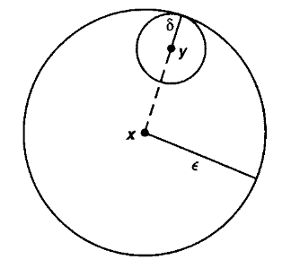
is said to be continuous at a point if for every there exists such that
or equivalently such that
where denotes the open ball (definition ).
The function is called just continuous if it is continuous at every point .
We now reformulate this analytic concept in terms of the simple but important concept of open sets:
Definition
(open ball)
Let , be a metric space. Then for every element and every a positive real number, write
Definition
(neighbourhood and open set)
Let be a metric space (def. ). Say that
-
A neighbourhood of a point is a subset which contains some open ball around (def. ).
-
An open subset of is a subset such that for every it also contains a neighbourhood of .
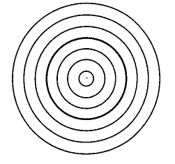
The following picture shows a point , some open balls containing it, and two of its neighbourhoods :
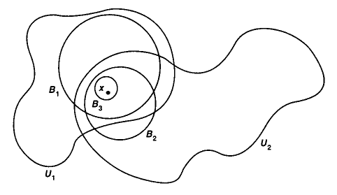
graphics grabbed from Munkres 75
Proposition
(rephrasing continuity in terms of open sets)
A function between metric spaces (def. ) is continuous in the epsilontic sense of def. precisely if it has the property that its pre-images of open subsets of (in the sense of def. ) are open subsets of .
principle of continuity
Pre-Images of open subsets are open.
Proof
First assume that is continuous in the epsilontic sense. Then for any open subset and any point in the pre-image, we need to show that there exists a neighbourhood of in . But by assumption there exists an open ball with . Since this is true for all , by definition this means that is open in .
Conversely, assume that takes open subsets to open subsets. Then for every and an open ball around its image, we need to produce an open ball in its pre-image. But by assumption contains a neighbourhood of which by definition means that it contains such an open ball around .
Topological spaces
Therefore we should pay attention to open subsets. It turns out that the following closure property is what characterizes the concept:
Proposition
(closure properties of open sets in a metric space)
The collection of open subsets of a metric space as in def. has the following properties:
-
The intersection of any finite number of open subsets is again an open subset.
-
The union of any set of open subsets is again an open subset.
In particular
- the empty set is open (being the union of no subsets)
and
- the whole set itself is open (being the intersection of no subsets).
This motivates the following generalized definition:
Definition
(topological spaces)
Given a set , then a topology on is a collection of subsets of called the open subsets, hence a subset of the power set
such that this is closed under forming
-
finite intersections;
-
arbitrary unions.
A topological space is a set equipped with such a topology.
The following shows all the topologies on the 3-element set (up to permutation of elements)
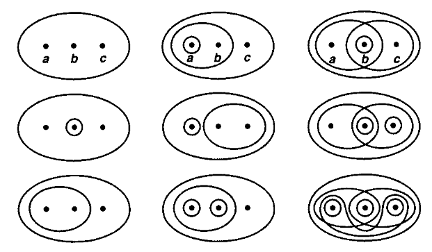
graphics grabbed from Munkres 75
It is now immediate to formally implement the
principle of continuity
Pre-Images of open subsets are open.
Definition
(continuous maps)
A continuous function between topological spaces
is a function between the underlying sets,
such that pre-images under of open subsets of are open subsets of .
The simple definition of open subsets and the simple principle of continuity gives topology its fundamental and universal flavor. The combinatorial nature of these definitions makes topology closely related to formal logic (for more on this see at locale).
Remark
(the category of topological spaces)
The composition of continuous functions is clearly associative and unital.
One says that
-
topological spaces constitute the objects
-
continuous maps constitute the morphisms (homomorphisms)
of a category. The category of topological spaces (“Top” for short).
It is useful to depict collections of objects with morphisms between them by diagrams, like this one:
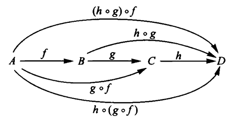
graphics grabbed from Lawvere-Schanuel 09.
Our motivating example now reads:
Example
(metric topology)
Let be a metric space. Then the collection of open subsets in def. constitutes a topology on the set , making it a topological space in the sense of def. . This is called the metric topology.
Stated more concisely: the open balls in a metric space constitute a “basis” for the metric topology.
One point of the general definition of “topological space” is that it admits constructions which intuitively should exist on “continuous spaces”, but which do not in general exist, for instance, as metric spaces:
Example
(discrete topological space)
For a bare set, then the discrete topology on regards every subset of as an open subset.
Example
(subspace topology)
Let be a topological space, and let be a subset of the underlying set. Then the corresponding topological subspace has as its underlying set, and its open subsets are those subsets of which arise as restrictions of open subsets of .
(Also called the initial topology of the inclusion map.)
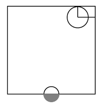
The picture on the right shows two open subsets inside the square, regarded as a topological subspace of the plane :
graphics grabbed from Munkres 75
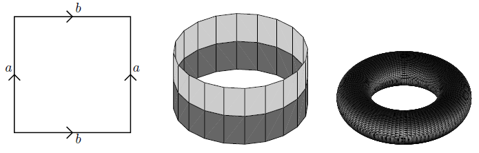
Example
(quotient topological space)
Let be a topological space (def. ) and let
be an equivalence relation on its underlying set. Then the quotient topological space has
- as underlying set the quotient set , hence the set of equivalence classes,
and
-
a subset is declared to be an open subset precisely if its preimage under the canonical projection map
is open in .
(This is also called the final topology of the projection .)
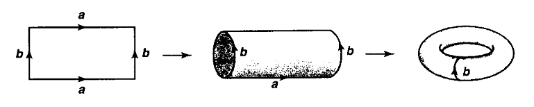
The above picture shows on the left the square (a topological subspace of the plane), then in the middle the resulting quotient topological space obtained by identifying two opposite sides (the cylinder), and on the right the further quotient obtained by identifying the remaining sides (the torus).
graphics grabbed from Munkres 75
Example
(product topological space)
For and two topological spaces, then the product topological space has
- as underlying set the Cartesian product of the underlying sets of and ,
and
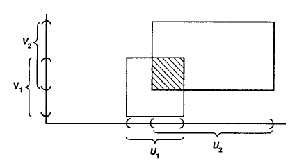
- its open sets are those subsets of the Cartesian product such that for all point there exists open sets and such that .
graphics grabbed from Munkres 75
These constructions of discrete topological spaces, quotient topological spaces, topological subspaces and of product topological spaces are simple examples of limits and of colimits of topological spaces. The category Top of topological spaces has the convenient property that all limits and colimits (over small diagrams) exist in it. (For more on this see at Top – Universal constructions.)
Homeomorphism
With the objects (topological spaces) and the morphisms (continuous maps) of the category Top of topology thus defined, we obtain the concept of “sameness” in topology.
To make this precise, one says that a morphism
in a category is an isomorphism if there exists a morphism going the other way around
which is an inverse in the sense that
Definition
(homeomorphisms)
An isomorphism in the category Top of topological spaces with continuous functions between them is called a homeomorphism.
Hence this is a continuous function
such that there exists an inverse morphism, namely a continuous function the other way around
such that
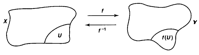
graphics grabbed from Munkres 75
Example
(open interval homeomorphic to the real line)
The open interval is homeomorphic to all of the real line
An inverse pair of continuous functions is for instance given by
and
Generally, every open ball in (def. ) is homeomorphic to all of .
Example
(interval glued at endpoints is homeomorphic to the circle)
As topological spaces, the interval with its two endpoints identified is homeomorphic (def. ) to the standard circle:
More in detail: let
be the unit circle in the plane
equipped with the subspace topology (example ) of the plane , which itself equipped with its standard metric topology (example ).
Moreover, let
be the quotient topological space (example ) obtained from the interval with its subspace topology by applying the equivalence relation which identifies the two endpoints (and nothing else).
Consider then the function
given by
This has the property that , so that it descends to the quotient topological space
We claim that is a homeomorphism (definition ).
First of all it is immediate that is a continuous function. This follows immediately from the fact that is a continuous function and by definition of the quotient topology (example ).
So we need to check that has a continuous inverse function. Clearly the restriction of itself to the open interval has a continuous inverse. It fails to have a continuous inverse on and on and fails to have an inverse at all on [0,1], due to the fact that . But the relation quotiented out in is exactly such as to fix this failure.
Similarly:
The square with two of its sides identified is the cylinder, and with also the other two sides identified is the torus:
If the sides are identified with opposite orientation, the result is the Möbius strip:
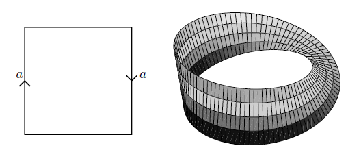
graphics grabbed from Lawson 03
Important examples of pairs of spaces that are not homeomorphic include the following:
Theorem
(topological invariance of dimension)
For but , then the Cartesian spaces and are not homeomorphic.
More generally, an open set in is never homeomorphic to an open set in if .
The proof of theorem is surprisingly hard, given how obvious the statement seems intuitively. It requires tools from a field called algebraic topology (notably Brouwer's fixed point theorem).
We showcase some basic tools of algebraic topology now and demonstrate the nature of their usage by proving two very simple special cases of the topological invariance of dimension (prop. and prop. below).
Example
(homeomorphism classes of surfaces)
The 2-sphere is not homeomorphic to the torus .
Generally the homeomorphism class of a closed orientable surface is determined by the number of “holes” it has, its genus.
Homotopy
We have seen above that for then the open ball in is not homeomorphic to, notably, the point (example , theorem ). Nevertheless, intuitively the -ball is a “continuous deformation” of the point, obtained as the radius of the -ball tends to zero.
This intuition is made precise by observing that there is a continuous function out of the product topological space (example ) of the open ball with the closed interval
which is given by rescaling:
This continuously interpolates between the open ball and the point in that for then it restricts to the defining inclusion , while for then it restricts to the map constant on the origin.
We may summarize this situation by saying that there is a diagram of continuous functions of the form
Such “continuous deformations” are called homotopies:
Definition
(homotopy)
For two continuous functions between topological spaces , then a (left) homotopy
is a continuous function
out of the product topological space (example ) of the open ball with the standard interval, such that this fits into a commuting diagram of the form
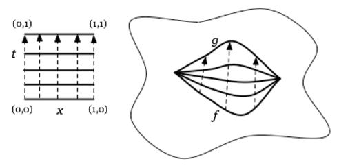
graphics grabbed from J. Tauber here
Definition
(homotopy equivalence)
A continuous function is called a homotopy equivalence if
-
there exists a continuous function the other way around, , and
-
left homotopies, def. , from the two composites to the identity:
and
Example
(open ball is contractible)
Any open ball (or closed ball), hence (by example ) any Cartesian space is homotopy equivalent to the point
Example
The following three graphs
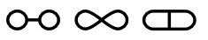
(i.e. the evident topological subspaces of the plane that these pictures indicate) are not homeomorphic. But they are homotopy equivalent, in fact they are each homotopy equivalent to the disk with two points removed, by the homotopies indicated by the following pictures:
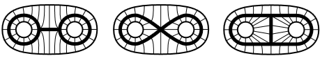
graphics grabbed from Hatcher
Connected components
Using the concept of homotopy one obtains the basic tool of algebraic topology, namely the construction of algebraic homotopy invariants of topological spaces. We introduce the simplest and indicate their use.
Definition
(connected components)
The set of homotopy classes of points in a topological space is called its set of path-connected components, denoted.
If consists of a single element, we say that is a path-connected topological space.
If is a continuous map between topological spaces, then on homotopy classes of points it induces a function between the corresponding connected components, which we denote by:
This construction is evidently compatible with composition, in that
and it evidently is unital, in that
One summarizes this by saying that is a functor from the category Top of topological spaces to the category Set of sets, denoted
An immediate but important consequence is this:
Proposition
If two topological spaces have sets of connected components that are not in bijection, then those spaces are not homeomorphic to each other:
Proof
Since is functorial, it immediately follows that it sends isomorphisms to isomorphisms, hence homeomorphisms to bijections:
This means that we may use path connected components as a first “topological invariant” that allows us to distinguish some topological spaces.
principle of algebraic topology
Use topological invariants to distinguish topological spaces.
As an example for how this is being used, we have the following proof of a simple special case of the topological invariance of dimension (theorem ):
Proposition
(topological invariance of dimension – first simple case)
The Cartesian spaces and are not homeomorphic (def. ).
Proof
Assume there were a homeomorphism
we will derive a contradiction. If is a homeomorphism, then clearly so is its restriction to the topological subspaces (example ) obtained by removing and .
It follows that we would get a bijection of connected components between and . But clearly the first set has two elements, while the second has just one:
The key lesson of the proof of prop. is its strategy:
principle of algebraic topology
Use topological invariants to distinguish topological spaces.
Of course in practice one uses more sophisticated invariants than just .
The next topological invariant after the connected components is the fundamental group:
Fundamental group
Definition
(fundamental group)
Let be a topological space and let be a chosen point. Then write
for, to start with, the set of homotopy classes of paths in that start and end at . Such paths are also called the continuous loops in based at .
-
Under concatenation of loops, becomes a semi-group.
-
The constant loop is a neutral element under this composition (thus making a “monoid”).
-
The reverse of a loop is its inverse in , making indeed into a group.
This is called the fundamental group of at .
The following picture indicates the four non-equivalent non-trivial generators of the fundamental group of the oriented surface of genus 2:
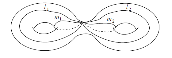
graphics grabbed from Lawson 03
Again, this operation is functorial, now on the category of pointed topological spaces, whose objects are topological spaces equipped with a chosen point, and whose morphisms are continuous maps that take the chosen basepoint of to that of :
As , so also is a topological invariant. As before, we may use this to prove a simple case of the theorem of the topological invariance of dimension:
Definition
A topological space for which
-
(path connected, def. )
-
(the fundamental group is trivial, def. ),
is called simply connected.
Proposition
(topological invariance of dimension – second simple case)
There is no homeomorphism between and .
Proof
Assume there were such a homeomorphism ; we will derive a contradiction.
If is a homeomorphism, then so is its restriction to removing the origin from and from :
Thse two spaces are both path-connected, hence does not distiguish them.
But they do have different fundamental groups :
-
The fundamental group of is (counting the winding of loops around the removed point). We discuss this further below in example .
-
The fundamental group of is trivial: because the single removed point is no obstruction to sliding loops past it and contracting them.
But since passing to fundamental groups is functorial, the same argument as in the proof of prop. shows that cannot be an isomorphism, hence not a homeomorphism.
We now discuss a “dual incarnation” of fundamental groups, which often helps to compute them.
Covering spaces
Definition
(covering space)
A covering space of a topological space is a continuous map
such that there exists an open cover , such that restricted to each then is homeomorphic over to the product topological space (example ) of with the discrete topological space (example ) on a set
For a point, then the elements in are called the leaves of the covering at .
Example
(covering of circle by circle)
Regard the circle as the topological subspace of elements of unit absolute value in the complex plane. For , consider the continuous function
given by taking a complex number to its th power. This may be thought of as the result of “winding the circle times around itself”. Precisely, for this is a covering space (def. ) with leaves at each point.
graphics grabbed from Hatcher
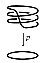
Example
(covering of circle by real line)
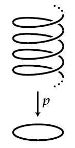
Consider the continuous function
from the real line to the circle, which,
-
with the circle regarded as the unit circle in the complex plane , is given by
-
with the circle regarded as the unit circle in , is given by
We may think of this as the result of “winding the line around the circle ad infinitum”. Precisely, this is a covering space (def. ) with the leaves at each point forming the set of natural numbers.
Definition
(action of fundamental group on fibers of covering)
Let be a covering space (def. )
Then for any point, and any choice of element of the leaf space over , there is, up to homotopy, a unique way to lift a representative path in of an element of the the fundamental group (def. ) to a continuous path in that starts at . This path necessarily ends at some (other) point in the same fiber. This construction provides a function
from the Cartesian product of the leaf space with the fundamental group. This function is compatible with the group-structure on , in that the following diagrams commute:
and
One says that is an action or permutation representation of on .
For any group, then there is a category whose objects are sets equipped with an action of , and whose morphisms are functions which respect these actions. The above construction yields a functor
Example
(three-sheeted covers of the circle)
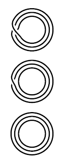
There are, up to isomorphism, three different 3-sheeted covering spaces of the circle .
The one from example for . Another one. And the trivial one. Their corresponding permutation actions may be seen from the pictures on the right.
graphics grabbed from Hatcher
We are now ready to state the main theorem about the fundamental group. Except that it does require the following slightly technical condition on the base topological space. This condition is satisfied for all “reasonable” topological spaces:
Definition
(semi-locally simply connected)
A topological space is called
-
locally path-connected if for every point and for every neighbourhood there exists a neighbourhood such that is path-connected (def. );
-
semi-locally simply connected if every point has a neighbourhood such that the induced morphism of fundamental groups is trivial (i.e. sends everything to the neutral element).
Theorem
(fundamental theorem of covering spaces)
Let be a topological space which is path-connected (def. ), locally path connected (def. ) and semi-locally simply connected (def. ). Then for any the functor
from def. that describes the action of the fundamental group of on the set of leaves over has the following property:
-
every isomorphism class of -actions is in the image of the functor (one says: the functor is essentially surjective);
-
for any two covering spaces of then the map on morphism sets
is a bijection (one says the functor is a fully faithful functor ).
A functor with these two properties one calls an equivalence of categories:
This has some interesting implications:
Every sufficiently nice topological space as above has a covering which is simply connected (def. ). This is the covering corresponding, under the fundamental theorem of covering spaces (theorem ) to the action of on itself. This is called the universal covering space . The above theorem implies that the fundamental group itself may be recovered as the automorphisms of the universal covering space:
Example
(computing the fundamental group of the circle)
The covering from example is simply connected (def. ), hence must be the universal covering space, up to homeomorphism.
It is fairly straightforward to see that the only homeomorphisms from to itself over are given by integer translations by :
Hence
and hence the fundamental group of the circle is the additive group of integers:
Basic facts
Central theorems
Related entries
The following is an (incomplete) list of available Lab entries related to topology.
Topological spaces
-
topological space, continuous map, homeomorphism, neighborhood
-
pointed space, contractible space, connected space, second countable space
-
convergence space, pretopological space, pseudotopological space, coarse topology
-
metric space, filtered space, connected filtered space, complete space, net, Polish space
-
separation axioms, Hausdorff space, regular space, normal space
-
compact space, locally compact space, compactum, paracompact space
-
convenient category of topological spaces, compactly generated space
See also examples in topology.
Manifolds and generalizations
-
manifold, smooth manifold, generalized smooth space, diffeological space, smooth space, Froelicher space
-
differential topology, microbundle, cobordism, derived smooth manifold
Algebraic topology and homotopy theory
-
homotopy, homotopy inverse, homotopy theory, homotopy equivalence, rational homotopy theory
-
model category, category of fibrant objects, Quillen adjunction, Quillen equivalence, category with weak equivalences,
-
Reedy category, Reedy model structure, generalized Reedy category
-
model structure on chain complexes, model structure on crossed complexes
-
homotopy hypothesis, homotopy theory of Grothendieck, test category
-
homotopy limit, homotopy colimit, homotopy pullback, homotopy image, homotopy coherent category theory, homotopy coherent nerve, Brown representability theorem
-
homotopy type, homotopy 1-type, homotopy 2-type, homotopy 3-type, homotopy n-type
-
fundamental group, homotopy group, suspension, Freudenthal suspension theorem, delooping
Topological homotopy theory
-
principal bundle, fiber bundle, vector bundle, principal 2-bundle, trivial bundle
-
fibration, Hurewicz fibration, Hurewicz connection, homotopy lifting property, Dold fibration
-
homotopy extension property, Hurewicz cofibration, deformation retract, model structure on topological spaces, Strøm's theorem
-
cocylinder, cylinder object, path object, mapping cone, path groupoid, path n-groupoid, fundamental groupoid
-
classifying space, Eilenberg-MacLane space,Moore space, Moore path category
-
spectrum, smash product of spectra, symmetric spectrum, stable (infinity,1)-category, commutative ring spectrum
Simplicial homotopy theory
-
simplicial set, simplex category, simplicial identities, simplicial object, cosimplicial object
-
boundary of a simplex, simplicial skeleton, category of simplices
-
combinatorial spectrum, simplicial groupoid, simplicial model category
-
simplicially enriched category, quasicategory, Segal category, complete Segal space
-
Kan fibration, Kan complex, nerve, nerve and realization, simplicial homotopy, simplicial homotopy group, simplicial local system
-
simplicial presheaf, local model structure on simplicial presheaves, local model structure on simplicial sheaves
-
marked simplicial set, model structure on marked simplicial over-sets, infinity topos, Higher Topos Theory
-
dendroidal set, model structure on dendroidal sets, cubical set, cellular set, cyclic object, Theta space
Sheaves, stacks, cohomology
- site, sheaf, flabby sheaf, local epimorphism, etale space, hypercover
- topos
- cohomology, sheaf cohomology, abelian sheaf cohomology, local system, category of sheaves
- Čech cohomology, Bredon cohomology, twisted cohomology, twisting cochain
- nonabelian algebraic topology, nonabelian cocycle, nonabelian cohomology
- principal infinity-bundle, BrownAHT, category of fibrant objects
- topological K-theory, gerbe, twisted K-theory, Karoubi K-theory, differential K-theory, K-theory spectrum
- de Rham cohomology, string topology
- Thom space, Thom bundle?, fiber integration, equivariant cohomology
- Poincaré duality, Spanier-Whitehead duality
- generalized cohomology, generalized (Eilenberg-Steenrod) cohomology, generalized (Eilenberg-Steenrod) homotopy
- topological stack, orbispace
- topological quantum field theory, tmf, cobordism hypothesis, topological T-duality
- characteristic class, Chern-Weil theory
Non-commutative topology
Topological physics
In string theory:
Computational Topology
References
Historical origins
The general idea of topology goes back to:
- Henri Poincaré, Analysis Situs, Journal de l’École Polytechnique 2 1 (1895) 1–123 [gallica:12148/bpt6k4337198/f7, Engl: pdf, pdf]
The notion of topological space involving neighbourhoods was first developed, for the special case now known as Hausdorff spaces, in:
- Felix Hausdorff, Grundzüge der Mengenlehre, Leipzig: Veit (1914), Reprinted by Chelsea Publishing Company (1944, 1949, 1965) [ISBN:978-0-8284-0061-9, ark:/13960/t2891gn8g]
The more general definition – dropping Hausdorff’s -separation axiom and formulated in terms of closure operators that preserve finite unions – is due to:
- Kazimierz Kuratowski, Sur l’opération Ā de l’Analysis Situs, Fundamenta Mathematicae 3 (1922) 182–199 [doi:10.4064/fm-3-1-182-199]
The modern formulation via open set was widely popularized by:
-
Nicolas Bourbaki], Eléments de mathématique II. Première partie. Les structures fondamentales de l’analyse. Livre III. Topologie générale. Chapitre I. Structures topologiques. Actualités scientifiques et industrielles, vol. 858. Hermann, Paris (1940)
General topology, Elements of Mathematics III, Springer (1971, 1990, 1995) [doi:10.1007/978-3-642-61701-0]
Further
Further textbook accounts:
-
John Kelley, General topology, D. van Nostrand, New York (1955), reprinted as: Graduate Texts in Mathematics, Springer (1975) [ISBN:978-0-387-90125-1]
-
James Dugundji, Topology, Allyn and Bacon 1966 (pdf)
-
James Munkres, Topology, Prentice Hall (1975, 2000) [ISBN:0-13-181629-2, pdf]
-
Richard E. Hodel (ed.), Set-Theoretic Topology, Academic Press (1977) [doi:10.1016/C2013-0-11355-4]
-
Klaus Jänich, Topology, Undergraduate Texts in Mathematics, Springer (1984, 1999) [ISBN:9780387908922, doi:10.1007/978-3-662-10574-0, Chapters 1-2: pdf]
-
Ryszard Engelking, General Topology, Sigma series in pure mathematics 6, Heldermann 1989 (ISBN 388538-006-4)
-
Steven Vickers, Topology via Logic, Cambridge University Press (1989) (toc pdf)
-
Glen Bredon, Topology and Geometry, Graduate texts in mathematics 139, Springer 1993 (doi:10.1007/978-1-4757-6848-0, pdf)
-
Terry Lawson, Topology: A Geometric Approach, Oxford University Press (2003) (pdf)
-
Anatole Katok, Alexey Sossinsky, Introduction to Modern Topology and Geometry (2010) [toc pdf, pdf]
and leading over to homotopy theory:
- Ioan Mackenzie James, General Topology and Homotopy Theory, Springer 1984
On counterexamples in topology:
- Lynn Arthur Steen, J. Arthur Seebach, Counterexamples in Topology, Springer 1971 (doi:10.1007/978-1-4612-6290-9)
With emphasis on category theoretic aspects of general topology, notably on -reflections:
-
Horst Herrlich, George Strecker, Categorical topology – Its origins as exemplified by the unfolding of the theory of topological reflections and coreflections before 1971 (pdf), pages 255-341 in: C. E. Aull, R Lowen (eds.), Handbook of the History of General Topology. Vol. 1, Kluwer 1997 (doi:10.1007/978-94-017-0468-7)
-
Tai-Danae Bradley, Tyler Bryson, John Terilla, Topology – A categorical approach, MIT Press 2020 (ISBN:9780262539357, web version)
See also:
-
Neil Strickland, A Bestiary of Topological Objects [pdf, pdf]
and see further references at algebraic topology.
Lecture notes:
-
Friedhelm Waldhausen, Topologie (pdf)
-
Alex Kuronya, Introduction to topology, 2010 (pdf)
-
Anatole Katok, Alexey Sossinsky, Introduction to modern topology and geometry (pdf)
-
Urs Schreiber, Introduction to Topology, Bonn 2017
-
Michael Müger, Topology for the working mathematician, Nijmegen 2018 (pdf)
Basic topology set up in intuitionistic mathematics is discussed in
- Franka Waaldijk, modern intuitionistic topology, 1996 (pdf)
See also:
- Topospaces, a Wiki with basic material on topology.
Last revised on November 28, 2023 at 11:30:28. See the history of this page for a list of all contributions to it.