nLab generalized (Eilenberg-Steenrod) cohomology
Context
Cohomology
Special and general types
-
group cohomology, nonabelian group cohomology, Lie group cohomology
-
-
cohomology with constant coefficients / with a local system of coefficients
Special notions
Variants
-
differential cohomology
Extra structure
Operations
Theorems
Homotopy theory
homotopy theory, (∞,1)-category theory, homotopy type theory
flavors: stable, equivariant, rational, p-adic, proper, geometric, cohesive, directed…
models: topological, simplicial, localic, …
see also algebraic topology
Introductions
Definitions
Paths and cylinders
Homotopy groups
Basic facts
Theorems
Contents
Idea
The collection of functors from (pointed) topological spaces to abelian groups which assign cohomology groups of ordinary cohomology (e.g. singular cohomology) may be axiomatized by a small set of natural conditions, called the Eilenberg-Steenrod axioms (Eilenberg-Steenrod 52, I.3), see below. One of these conditions, the “dimension axiom” (Eilenberg-Steenrod 52, I.3 Axiom 7) says that the (co)homology groups assigned to the point are concentrated in degree 0. The class of functors obtained by discarding this “dimension axiom” came to be known as generalized (co)homology theories (Whitehead 62) or extraordinary (co)homology theories.
Examples include topological K-theory (Atiyah-Hirzebruch 61, 1.8), elliptic cohomology and cobordism cohomology theory. Dually one speaks of generalized homology.
Notice that, while the terminology “generalized cohomology” is standard in algebraic topology with an eye towards stable homotopy theory, it is somewhat unfortunate in that there are various other and further generalizations of the axioms that all still deserve to be and are called “cohomology”. For instance dropping the suspension axiom leads to nonabelian cohomology and dropping the “homotopy axiom” (and taking the domain spaces to be smooth manifolds) leads to the further generality of differential cohomology. This entry here is concerned with the generalization obtained from the Eilenberg-Steenrod axioms by just discarding the dimension axiom. For lack of a better term, we say “generalized (Eilenberg-Steenrod) cohomology” here.
In (Whitehead 62) it was observed that every spectrum induces a generalized homology theory. The Brown representability theorem (Brown 62) asserts that every generalized (co)homology arises this way, being represented by mapping spectra into/smash product with a spectrum. But beware that the cohomology theory represented by a spectrum in general contains strictly less information than the spectrum, due to the existence of “phantom maps”.
On the other hand, if one refines the concept of a generalized homology theory from taking values in graded abelian? groups to taking values in homotopy types then it does become equivalent to the concept of spectrum, this is the statement at excisive functor – Examples – Spectrum objects.
This means that from a perspective of higher category theory, generalized Eilenberg-Steenrod cohomology is the intrinsic cohomology of the (∞,1)-category of spectra, or better: twisted generalized Eilenberg-Steenrod cohomology is the intrinsic cohomology of the tangent (∞,1)-topos of parameterized spectra.
Generalized Eilenberg-Steenrod cohomology is cohomology with coefficients a spectrum object.
Definition
This sections states the classical formulation of the Eilenberg-Steenrod axioms due to (Eilenberg-Steenrod 52, I.3) in terms of concepts from classical algebraic topology, such as CW-pairs and mapping cones.
More abstractly, via the classical model structure on topological spaces, these structures are seen to serve as presentations for certain homotopy pushouts. In terms of “abstract homotopy theory” ((infinity,1)-category theory) one obtains a more streamlined formulation, which we turn to below.
There are two versions of the statement of the axioms:
There are functors taking any reduced cohomology theory to an unreduced one, and vice versa. When some fine detail in the axioms is suitably set up, then this establishes an equivalence between reduced and unreduced generalized cohomology:
The fine detail in the axioms that makes this work is such as to ensure that a cohomology theory is a functor on the opposite of the (pointed/pairwise) classical homotopy category. Since this has different presentations, there are corresponding different versions of suitable axioms:
-
On the one hand, may be presented by topological spaces homeomorphic to CW-complexes and with homotopy equivalence-classes of continuous functions between them, and accordingly a generalized cohomology theory may be taken to be a funtor on (pointed/pairs of) CW-complexes invariant under homotopy equivalence.
-
On the other hand, may be presented by all topological spaces with weak homotopy equivalences inverted, and accordingly a generalized cohomology theory may be taken to be a functor on all (pointed/pairs of) topological spaces that sends weak homotopy equivalences to isomorphisms.
Notice however that “classical homotopy category” is already ambiguous. Pre Quillen this was the category of all topological spaces with homotopy equivalence classes of maps between them, and often generalized cohomology functors are defined on this larger category and only restricted to CW-complexes or required to preserve weak homotopy equivalences when need be (e.g. Switzer 75, p.117), such as for establishing the equivalence between reduced and unreduced theories.
Moreover, historically, these conditions have been decomposed in several numbers of ways. Notably (Eilenberg-Steenrod 52) originally listed 7 axioms for unreduced cohomology, more than typically counted today, but their axioms 1 and 2 jointly just said that we have a functor on topological spaces, axiom 3 was the condition for the connecting homomorphism to be a natural transformation, conditions which later (Switzer 75, p. 99,100) were absorbed in the underlying structure.
Finally, following the historical development it is common to state the exactness properties of cohomology functors in terms of mapping cone constructions. These are models for homotopy cofibers, but in general only when some technical conditions are met, such that the underlying topological spaces are CW-complexes.
For these reasons, in the following we stick to two points of views: where we discuss cohomology theories as functors on topological spaces we restrict attention to those homeomorphic to CW-complexes. In a second description we speak fully abstractly about functors on the homotopy category of a given model category of -category.
Reduced cohomology
Throughout, write Top for the category of topological spaces homeomorphic to CW-complexes. Write for the corresponding category of pointed topological spaces.
Recall (here) that colimits in are computed as colimits in Top (here) after adjoining the base point and its inclusion maps to the given diagram.
Example
The coproduct in pointed topological spaces is the wedge sum, denoted .
Write
for the reduced suspension functor.
Write for the category of integer-graded abelian groups.
Definition
A reduced cohomology theory is a functor (“pullback in cohomology”)
from the opposite of pointed topological spaces (CW-complexes) to -graded abelian groups (“cohomology groups”), in components
and equipped with a natural isomorphism of degree +1, to be called the suspension isomorphism, of the form
such that:
-
(homotopy invariance) If are two morphisms of pointed topological spaces such that there is a (base point preserving) homotopy between them, then the induced homomorphisms of abelian groups are equal
-
(exactness) For an inclusion of pointed topological spaces, with the induced mapping cone, then this gives an exact sequence of graded abelian groups
We say is additive if in addition
-
(wedge axiom) For any set of pointed CW-complexes, then the canonical comparison morphism
is an isomorphism, from the functor applied to their wedge sum, example , to the product of its values on the wedge summands, .
We say is ordinary if its value on the 0-sphere is concentrated in degree 0:
- (Dimension) .
A homomorphism of reduced cohomology theories
is a natural transformation between the underlying functors which is compatible with the suspension isomorphisms in that all the following squares commute
(e.g. AGP 02, def. 12.1.4)
We may rephrase this more intrinsically and more generally:
Definition
Let be an (∞,1)-category with (∞,1)-pushouts, and with a zero object . Write for the corresponding suspension (∞,1)-functor.
A reduced generalized cohomology theory on is
-
a functor
(from the opposite of the homotopy category of into -graded abelian groups);
-
a natural isomorphisms (“suspension isomorphisms”) of degree +1
such that
-
takes small coproducts to products;
-
takes homotopy cofiber sequences to exact sequences.
Definition
Given a generalized cohomology theory on some as in def. , and given a homotopy cofiber sequence in
then the corresponding connecting homomorphism is the composite
Proposition
The connecting homomorphisms of def. are part of long exact sequences
See at long exact sequence in generalized cohomology.
Proof
By the defining exactness of , def. , and the way this appears in def. , using that is by definition an isomorphism.
Unreduced cohomology
In the following a pair refers to a subspace inclusion of topological spaces (CW-complexes) . Whenever only one space is mentioned, the subspace is assumed to be the empty set . Write for the category of such pairs (the full subcategory of the arrow category of on the inclusions). We identify by .
Definition
A cohomology theory (unreduced, relative) is a functor
to the category of -graded abelian groups, as well as a natural transformation of degree +1, to be called the connecting homomorphism, of the form
such that:
-
(homotopy invariance) For a homotopy equivalence of pairs, then
is an isomorphism;
-
(exactness) For the induced sequence
is a long exact sequence of abelian groups.
-
(excision) For such that , then the natural inclusion of the pair induces an isomorphism
We say is additive if it takes coproducts to products:
-
(additivity) If is a coproduct, then the canonical comparison morphism
is an isomorphism from the value on to the product of values on the summands.
We say is ordinary if its value on the point is concentrated in degree 0
- (Dimension): .
A homomorphism of unreduced cohomology theories
is a natural transformation of the underlying functors that is compatible with the connecting homomorphisms, hence such that all these squares commute:
e.g. (AGP 02, def. 12.1.1).
Lemma
The excision axiom in def. is equivalent to the following statement:
For all with , then the inclusion
induces an isomorphism,
(e.g Switzer 75, 7.2)
Proof
In one direction, suppose that satisfies the original excision axiom. Given with , set and observe that
and that
Hence the excision axiom implies .
Conversely, suppose satisfies the alternative condition. Given with , observe that we have a cover
and that
Hence
The following lemma shows that the dependence in pairs of spaces in a generalized cohomology theory is really a stand-in for evaluation on homotopy cofibers of inclusions.
Lemma
Let be an cohomology theory, def. , and let . Then there is an isomorphism
between the value of on the pair and its value on the mapping cone of the inclusion, relative to a basepoint.
If moreover is (the retract of) a relative cell complex inclusion, then also the morphism in cohomology induced from the quotient map is an isomorphism:
(e.g AGP 02, corollary 12.1.10)
Proof
Consider , the cone on minus the base . We have
and hence the first isomorphism in the statement is given by the excision axiom followed by homotopy invariance (along the contraction of the cone to the point).
Next consider the quotient of the mapping cone of the inclusion:
If is a cofibration, then this is a homotopy equivalence since is contractible and since by the dual factorization lemma is a weak homotopy equivalence, hence a homotopy equivalence on CW-complexes.
Hence now we get a composite isomorphism
Example
As an important special case of : Let be a pointed CW-complex. For the quotient map from the reduced cone on to the reduced suspension, then
is an isomorphism.
Proposition
(exact sequence of a triple)
For an unreduced generalized cohomology theory, def. , then every inclusion of two consecutive subspaces
induces a long exact sequence of cohomology groups of the form
where
Proof
Apply the braid lemma to the interlocking long exact sequences of the three pairs , , . See here for details.
The dual braid diagram for generalized homology is this:
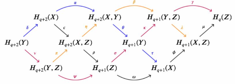
(graphics from this Maths.SE comment)
Remark
The exact sequence of a triple in prop. is what gives rise to the Cartan-Eilenberg spectral sequence for -cohomology of a CW-complex .
Example
For a pointed topological space and its reduced cone, the long exact sequence of the triple , prop. ,
exhibits the connecting homomorphism here as an isomorphism
This is the suspension isomorphism extracted from the unreduced cohomology theory, see def. below.
Proposition
Given an unreduced cohomology theory, def. . Given a topological space covered by the interior of two spaces as , then for each there is a long exact sequence of cohomology groups of the form
e.g. (Switzer 75, theorem 7.19, Aguilar-Gitler-Prieto 02, theorem 12.1.22, see also at Brown-Gersten property)
Relation between reduced and unreduced cohomology
Definition
(unreduced to reduced cohomology)
Let be an unreduced cohomology theory, def. . Define a reduced cohomology theory, def. as follows.
For a pointed topological space, set
This is clearly functorial. Take the suspension isomorphism to be the composite
of the isomorphism from example and the inverse of the isomorphism from example .
(e.g. Switzer 75, 7.34)
Proof
We need to check the exactness axiom given any . By lemma we have an isomorphism
Unwinding the constructions shows that this makes the following diagram commute:
where the vertical sequence on the right is exact by prop. . Hence the left vertical sequence is exact.
Definition
(reduced to unreduced cohomology)
Let be a reduced cohomology theory, def. . Define an unreduced cohomolog theory , def. , by
e.g. (Switzer 75, 7.35)
Proof
Exactness holds by prop. . For excision, it is sufficient to consider the alternative formulation of lemma . For CW-inclusions, this follows immediately with lemma .
Theorem
The constructions of def. and def. constitute a pair of functors between then categories of reduced cohomology theories, def. and unreduced cohomology theories, def. which exhbit an equivalence of categories.
Proof
(…careful with checking the respect for suspension iso and connecting homomorphism..)
To see that there are natural isomorphisms relating the two composites of these two functors to the identity:
One composite is
where on the right we have, from the construction, the reduced mapping cone of the original inclusion with a base point adjoined. That however is isomorphic to the unreduced mapping cone of the original inclusion. With this the natural isomorphism is given by lemma .
The other composite is
where on the right we have the reduced mapping cone of the point inclusion with a point adoined. As before, this is isomorphic to the unreduced mapping cone of the point inclusion. That finally is clearly homotopy equivalent to , and so now the natural isomorphism follows with homotopy invariance.
Finally we record the following basic relation between reduced and unreduced cohomology:
Proposition
Let be an unreduced cohomology theory, and its reduced cohomology theory from def. . For a pointed topological space, then there is an identification
of the unreduced cohomology of with the direct sum of the reduced cohomology of and the unreduced cohomology of the base point.
Proof
The pair induces the sequence
which by the exactness clause in def. is exact.
Now since the composite is the identity, the morphism has a section and so is in particular an epimorphism. Therefore, by exactness, the connecting homomorphism vanishes, and we have a short exact sequence
with the right map an epimorphism. Hence this is a split exact sequence and the statement follows.
Brown functoriality
Proposition
Given a generalized cohomology functor , def. , its underlying Set-valued functors are Brown functors, def. .
Proof
The first condition on a Brown functor holds by definition of . For the second condition, given a homotopy pushout square
in , consider the induced morphism of the long exact sequences given by prop.
Here the outer vertical morphisms are isomorphisms, as shown, due to the pasting law (see also at fiberwise recognition of stable homotopy pushouts).
This means that the four lemma applies to this diagram. Inspection shows that this implies the claim.
Examples
Properties
Expression by ordinary cohomology via Atiyah-Hirzebruch spectral sequence
The Atiyah-Hirzebruch spectral sequence serves to express generalized cohomology in terms of ordinary cohomology with coefficients in .
Whitehead theorem
Proposition
Let be a morphism of reduced generalized (co-)homology functors, def. (a natural transformation) such that its component
on the 0-sphere is an isomorphism. Then is an isomorphism for any CW-complex with a finite number of cells. If both and satisfy the wedge axiom, then is an isomorphism for any CW-complex, not necessarily finite.
For and ordinary cohomology/ordinary homology functors a proof of this is in (Eilenberg-Steenrod 52, section III.10). From this the general statement follows (e.g. Kochman 96, theorem 3.4.3, corollary 4.2.8) via the naturality of the Atiyah-Hirzebruch spectral sequence (the classical result gives that induces an isomorphism between the second pages of the AHSSs for and ). A complete proof of the general result is also given as (Switzer 75, theorem 7.55, theorem 7.67)
Related concepts
twisted generalized cohomology theory is conjecturally ∞-categorical semantics of linear homotopy type theory:
References
The original article on the Eilenberg–Steenrod axioms:
- Samuel Eilenberg, Norman E. Steenrod, Axiomatic Approach to Homology Theory, Proceedings of the National Academy of Sciences 31 4 (1945) 117–120 [doi:10.1073/pnas.31.4.117]
Further development and an expository account:
- Samuel Eilenberg, Norman Steenrod, Foundations of algebraic topology, Princeton 1952 (pdf, ISBN:9780691653297)
The concept of generalized homology obtained by discarding the dimension axiom and the observation that every spectrum induces an example is due to
- George Whitehead, Generalized homology theories, Transactions of the American Mathematical Society, 102 (1962) 227-283 (pdf, jstor:1993676)
The proof that every generalized (co)homology theory arises this way (Brown representability theorem) is due to
-
Edgar Brown, Cohomology theories, Annals of Mathematics, Second Series 75: 467–484 (1962) (jstor:1970209)
-
Edgar Brown, Abstract homotopy theory, Trans. AMS 119 no. 1 (1965) (doi:10.1090/S0002-9947-1965-0182970-6)
An early lecture note account is in
- Frank Adams, part III, sections 2 and 6 of Stable homotopy and generalised homology, 1974
Textbook accounts:
-
Robert Switzer, chapter 7 (and 8-12) of Algebraic Topology - Homotopy and Homology, Die Grundlehren der Mathematischen Wissenschaften in Einzeldarstellungen, Vol. 212, Springer-Verlag, New York, N. Y., 1975.
-
John Michael Boardman, Section 3 of: Stable Operations in Generalized Cohomology [pdf, pdf] in: Ioan Mackenzie James (ed.) Handbook of Algebraic Topology Oxford 1995 (doi:10.1016/B978-0-444-81779-2.X5000-7)
-
Stanley Kochman, section 3.4 of Bordism, Stable Homotopy and Adams Spectral Sequences, AMS 1996
-
Peter May chapter 18 of A Concise Course on Algebraic Topology, Chicago Lecture Notes 1999 (pdf)
-
Marcelo Aguilar, Samuel Gitler, Carlos Prieto, section 12.1 of Algebraic topology from a homotopical viewpoint, Springer (2002) (toc pdf)
-
Akira Kono, Dai Tamaki, Generalized cohomology, AMS 2002, esp. chapter 2 pdf, ISBN: 978-0-8218-3514-2
-
Stefan Schwede, chapter II, section 6 of Symmetric spectra, 2012 (pdf)
Discussion in the further generality of equivariant cohomology is in
- Tammo tom Dieck, section 7 of Transformation Groups and Representation Theory, Lecture Notes in Mathematics 766, Springer 1979
A pedagogical introduction to spectra and generalized (Eilenberg-Steenrod) cohomology is in
Formulation in (infinity,1)-category theory is in
- Jacob Lurie, section 1.4.1 of Higher Algebra
More references relating to the nPOV on cohomology include:
-
Mike Hopkins, Complex oriented cohomology theories and the language of stacks course notes (pdf)
-
Jacob Lurie, A Survey of Elliptic Cohomology - cohomology theories
Formulation in homotopy type theory (cf. cohomology in homotopy type theory):
-
Evan Cavallo, Section 3.2 of: Synthetic Cohomology in Homotopy Type Theory (2015) [pdf, pdf]
-
Floris van Doorn, around Def. 5.4.2 in: On the Formalization of Higher Inductive Types and Synthetic Homotopy Theory (2018) [arXiv:1808.10690, pdf]
Last revised on September 5, 2023 at 19:33:08. See the history of this page for a list of all contributions to it.