nLab mapping cone
Context
Limits and colimits
1-Categorical
2-Categorical
(∞,1)-Categorical
Model-categorical
Homotopy
homotopy theory, (∞,1)-category theory, homotopy type theory
flavors: stable, equivariant, rational, p-adic, proper, geometric, cohesive, directed…
models: topological, simplicial, localic, …
see also algebraic topology
Introductions
Definitions
Paths and cylinders
Homotopy groups
Basic facts
Theorems
Contents
Idea
The mapping cone of a morphism in some homotopical category (precisely: a category of cofibrant objects) is, if it exists, a particular representative of the homotopy cofiber of .
It is also called the homotopy cokernel of or the weak quotient of by the image of in under .
The dual notion is that of mapping cocone.
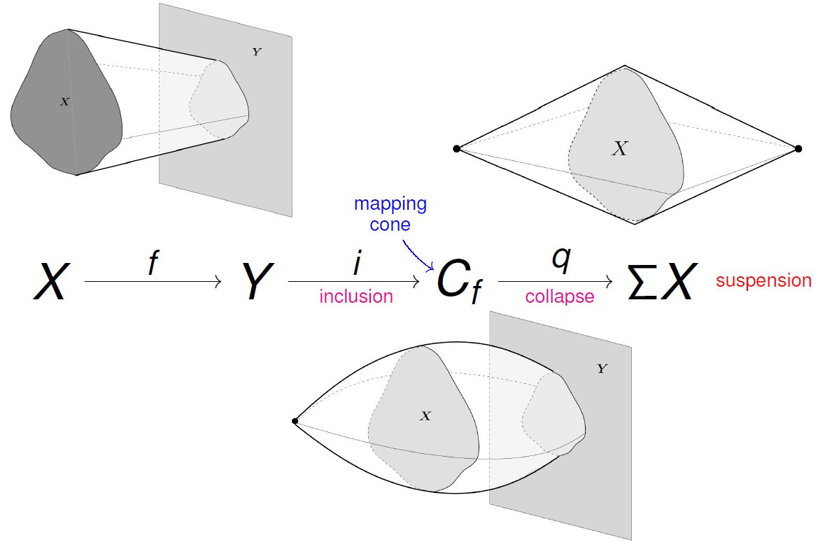
(graphics taken from Muro 2010)
Definition
The mapping cone construction is a means to present in a category with weak equivalences the following canonical construction in homotopy theory/(∞,1)-category theory.
Definition
In an (∞,1)-category with terminal object and (∞,1)-pushout, the homotopy cofiber of a morphism is the homotopy pushout
hence the object universal construction sitting universally in a diagram of the form
Proposition
If the (∞,1)-category is presented by (is equivalent to the simplicial localization of) a category of cofibrant objects (for instance given by the cofibrant objects in a model category) then this homotopy cofiber is presented by the ordinary colimit
in using any cylinder object for .
This is discussed in detail at factorization lemma and at homotopy pullback.
Remark
Intuitively this says that is the object obtained by
-
forming the cylinder over ;
-
gluing to one end of that the object as specified by the map .
-
shrinking the other end of the cylinder to the point.
Intuitively it is clear that this way every cycle in that happens to be in the image of can be “continuously” translated in the cylinder-direction, keeping it constant in , to the other end of the cylinder, where it becomes the point. This means that every homotopy group of in the image of vanishes in the mapping cone. Hence in the mapping cone the image of under in is removed up to homotopy. This makes it clear how is a homotopy-version of the cokernel of . And therefore the name “mapping cone”.
Remark
A morphism out of a cylinder object is a left homotopy between its restrictions and to the cylinder boundaries
Therefore prop. says that the mapping cone is the the universal object with a morphism from and a left homotopy from to the zero morphism. This is of course also precisely what def. is saying.
Proposition
The colimit in prop. may be computed in two stages by two consecutive pushouts in , and in two ways by the following pasting diagram:
Here every square is a pushout, (and so by the pasting law is every rectangular pasting composite).
This now is a basic fact in ordinary category theory. The pushouts appearing here go by the following names:
Definition
The pushout
defines the cone over (with respect to the chosen cylinder object): the result of taking the cylinder over and identifying one -shaped end with the point.
The pushout
defines the mapping cylinder of , the result of identifying one end of the cylinder over with , using as the gluing map.
The pushout
defines the mapping cone of : the result of forming the cylinder over and then identifying one end with the point and the other with , via .
The geometric intuition behind this is best seen in the archetypical example of the classical model structure on topological spaces. See the example For topological spaces below. The example For chain complexes can be understood similarly geometrically by thinking of all chain complexes as singular chains on topological spaces.
Examples
We discuss realizations of the general construction in various contexts. Some of these examples are regarded in parts of the literature as the default examples, notably that for topological spaces and that for chain complexes.
Suspension
The mapping cone of the morphism to the terminal object is the suspension object of an object . The dual notion of the loop space object of .
For topological spaces
The notion mapping cone derives its name from its geometrical interpretation in the category Top of topological spaces.
For more details see also at topological cofiber sequence.
With respect to the standard model structure on topological spaces every CW-complex is a cofibrant object, and hence mapping cones on maps between CW-complexes have intrinsic meaning in homotopy theory.
Write Top for the closed interval with its Euclidean metric topology. This is an interval object for the standard model structure. We may therefore take the cylinder object of a topological space to be
which is literally the cylinder over .
Given a continuous function , the topological space is
This is the disjoint union of with followed by an identification under which for each a point is identified with the point and followed by the contraction of to a point.
Of course the opposite convention is also possible: identify with for all and then contract to a point; the two constructions of cones are canonically homeomorphic; the first is sometimes called the “inverse mapping cone”.
The singular chain complex functor from Top to the category of chain complexes of abelian groups sends the mapping cone to a mapping cone in the sense of chain complexes (up to conventions on the orientation of the interval and vector order in the definition of mapping cone of chain complexes).
For chain complexes
Let be the category of chain complexes in Mod for some ring .
(For instance if the integers, then this is , chain complexes of abelian groups. More generally can be replaced by any abelian category in the following, with the evident changes in the presentation here and there.)
We derive an explicit presentation of the mapping cone of a chain map , according to the general definition . The end result is prop. below, reproducing the classical formula for the mapping cone.
Definition
Write for the chain complex concentrated on in degree 0
Remark
This may be understood as the normalized chain complex of chains of simplices on the terminal simplicial set , the 0-simplex.
Definition
Let be given by
Denote by
the chain map which in degree 0 is the canonical inclusion into the second summand of a direct sum and by
correspondingly the canonical inclusion into the first summand.
Remark
This is the standard interval object in chain complexes.
It is in fact the normalized chain complex of chains on a simplicial set for the canonical simplicial interval, the 1-simplex:
The differential here expresses the alternating face map complex boundary operator, which in terms of the three non-degenerate basis elements is given by
We decompose the proof of this statement is a sequence of substatements.
Proposition
For the tensor product of chain complexes
is a cylinder object of for the structure of a category of cofibrant objects on whose cofibrations are the monomorphisms and whose weak equivalences are the quasi-isomorphisms (the substructure of the standard injective model structure on chain complexes).
Proof
By the formula discussed at tensor product of chain complexes the components arise as the direct sum
and the differential picks up a sign when passed past the degree-1 term :
Remark
The two boundary inclusions of into the cylinder are given in terms of def. by
and
which in components is the inclusion of the second or first direct summand, respectively
One part of definition now reads:
Definition
For a chain map, the mapping cylinder is the pushout
Proof
The colimits in a category of chain complexes are computed in the underlying presheaf category of towers in . There they are computed degreewise in (see at limits in presheaf categories). Here the statement is evident:
the pushout identifies one direct summand with along and so where previously a appeared on the diagonl, there is now .
The last part of definition now reads:
In the literature this appears for instance as (Schapira, def. 3.2.2).
Proposition
The components of the mapping cone are
with differential given by
and hence in matrix calculus by
Proof
As before the pushout is computed degreewise. This identifies the remaining unshifted copy of with 0.
Proposition
For a chain map, the canonical inclusion of into the mapping cone of is given in components
by the canonical inclusion of a summand into a direct sum.
Proof
This follows by starting with remark and then following these inclusions through the formation of the two colimits as discussed above.
The construction above builds the mapping cone explicitly via the standard formula for homotopy pushouts. Often however other presentations are more convenient:
Proposition
For a chain map, consider the double complex concentrated in degrees and with .
Then the total complex of is also a model for the mapping cone of :
Proof
One checks by inspection that for for which there is a chain homotopy (given only by multiplication by signs).
This appears for instance as (Weibel, Exercise 1.2.8).
For cochain complexes
We spell out the situation in more detail in a category of cochain complexes.
Let be some concrete additive category and the category of chain complexes in . For
a morphism, the mapping cone is the complex
There is a canonical cochain homotopy
where is the canonical inclusion, componentwise given by
and where the cochain homotopy has components
which we denote on by
The fact that this is a cochain homotopy means that
which we check on any by computing
where we used the above definition of and the fact that is a chain homomorphism and hence intertwines the differentials.
This cochain homotopy is universal in that for any other cochain homotopy
hence
we have a morphism
given on by and on by
which is indeed a cochain homomorphism because for all we have
and which is unique with the property that whiskering of 2-morphisms gives
hence that
and
In additive categories with translation
Let be an additive category with translation . Let and be two differential objects in and any morphism in .
The mapping cone of is the differential object whose underlying object is the direct sum and whose differential is given in matrix calculus notation by
Notice the minus sign here, coming from the definition of a shifted differential object.
Properties
Homology exact sequences and fiber sequences
We discuss the relation between mapping cones in categories of chain complexes, as above, and long exact sequences in homology. For an exposition of the following see there the section Relation to homotopy fiber sequences.
Let be a chain map and write for its mapping cone as explicitly given in prop. .
Definition
Write for the suspension of a chain complex of . Write
for the chain map which in components
is given, via prop. , by the canonical projection out of a direct sum
Proposition
The chain map represents the homotopy cofiber of the canonical map .
Proof
By prop. and def. the sequence
is a short exact sequence of chain complexes (since it is so degreewise, in fact degreewise it is even a split exact sequence). In particular we have a cofiber pushout diagram
Now, in the injective model structure on chain complexes all chain complxes are cofibrant objects and an inclusion such as is a cofibration. By the detailed discussion at homotopy limit this means that the ordinary colimit here is in fact a homotopy colimit, hence exhibits as the homotopy cofiber of .
Corollary
For a chain map, there is a homotopy cofiber sequence of the form
In order to compare this to the discussion of connecting homomorphisms, we now turn attention to the case that happens to be a monomorphism. Notice that this we can always assume, up to quasi-isomorphism, for instance by prolonging by the map into its mapping cylinder
By the axioms on an abelian category in this case we have a short exact sequence
of chain complexes. The following discussion revolves around the fact that now as well as are both models for the homotopy cofiber of .
Lemma
Let
be a short exact sequence of chain complexes.
The collection of linear maps
constitutes a chain map
This is a quasi-isomorphism. The inverse of is given by sending a representing cycle to
where is any choice of lift through and where is the formula expressing the connecting homomorphism in terms of elements, as discussed at Connecting homomorphism – In terms of elements.
Finally, the morphism is eqivalent in the homotopy category (the derived category) to the zigzag
In the literature this appears for instance as (Schapira, cor. 7.2.2).
Proof
To see that defines a chain map recall the differential from prop. , which acts by
and use that is in the kernel of by exactness, hence
It is immediate to see that we have a commuting diagram of the form
since the composite morphism is the inclusion of followed by the bottom morphism on .
Abstractly, this already implies that is a quasi-isomorphism, for this diagram gives a morphism of cocones under the diagram defining in prop. and by the above both of these cocones are homotopy-colimiting.
But in checking the claimed inverse of the induced map on homology groups, we verify this also explicity:
We first determine those cycles which lift a cycle . By lemma a lift of chains is any pair of the form where is a lift of through . So has to be found such that this pair is a cycle. By prop. the differential acts on it by
and so the condition is that
(which implies due to the fact that is assumed to be an inclusion, hence that is the restriction of to elements in ).
This condition clearly has a unique solution for every lift and a lift always exists since is surjective, by assumption that we have a short exact sequence of chain complexes. This shows that is surjective.
To see that it is also injective we need to show that if a cycle maps to a cycle that is trivial in in that there is with , then also the original cycle was trivial in homology, in that there is with
For that let be a lift of through , which exists again by surjectivity of . Observe that
by assumption on and , and hence that is in by exactness.
Hence trivializes the given cocycle:
Theorem
Let
be a short exact sequence of chain complexes.
Then the chain homology functor
sends the homotopy cofiber sequence of , cor. , to the long exact sequence in homology induced by the given short exact sequence, hence to
where is the th connecting homomorphism.
Proof
By lemma the homotopy cofiber sequence is equivalen to the zigzag
Observe that
It is therefore sufficient to check that
equals the connecting homomorphism induced by the short exact sequence.
By prop. the inverse of the vertical map is given by choosing lifts and forming the corresponding element given by the connecting homomorphism. By prop. the horizontal map is just the projection, and hence the assignment is of the form
So in total the image of the zig-zag under homology sends
By the discussion there, this is indeed the action of the connecting homomorphism.
Distinguished triangles from mapping cones
In summary, the above says that for every chain map we obtain maps
which form a homotopy fiber sequence and such that this sequence continues by forming suspensions, hence for all we have
To amplify this quasi-cyclic behaviour one sometimes depicts the situation as follows:
and hence speaks of a “triangle”, or distinguished triangle or mapping cone triangle of .
- distinguished triangle = period of homotopy fiber sequence .
Due to these “triangles” one calls the homotopy category of chain complexes localized at the quasi-isomorphisms, hence the derived category, a triangulated category.
Notice that equivalently we can express the triangles via the mapping cylinder. For every map of chain complexes , the cylinder is quasi-isomorphic to , and moreover in the homotopy category of chain complexes, every distinguished triangle is quasi-isomorphic to a distinguished triangle of the form
for some where all the morphisms in the triangle are appropriatedly induced by .
Related concepts
examples of universal constructions of topological spaces:
References
In the context of chain complexes the construction is discussed for instance in
-
Pierre Schapira, section 3.2 and section 7 of Categories and homological algebra (2011) (pdf)
-
Charles Weibel, section 1.5 of An Introduction to Homological Algebra .
In the context of spectra discussion includes
- Robert Switzer, around 8. 17 of Algebraic Topology - Homotopy and Homology, Die Grundlehren der Mathematischen Wissenschaften in Einzeldarstellungen, Vol. 212, Springer-Verlag, New York, N. Y., 1975.
Graphics taken from
- Fernando Muro, Representability of Cohomology Theories, Joint Mathematical Conference CSASC 2010, 22–27 January 2010, Prague, Czech Republic (slides)
Last revised on December 8, 2023 at 16:11:36. See the history of this page for a list of all contributions to it.