nLab stereographic projection
Context
Spheres
Topology
topology (point-set topology, point-free topology)
see also differential topology, algebraic topology, functional analysis and topological homotopy theory
Basic concepts
-
fiber space, space attachment
Extra stuff, structure, properties
-
Kolmogorov space, Hausdorff space, regular space, normal space
-
sequentially compact, countably compact, locally compact, sigma-compact, paracompact, countably paracompact, strongly compact
Examples
Basic statements
-
closed subspaces of compact Hausdorff spaces are equivalently compact subspaces
-
open subspaces of compact Hausdorff spaces are locally compact
-
compact spaces equivalently have converging subnet of every net
-
continuous metric space valued function on compact metric space is uniformly continuous
-
paracompact Hausdorff spaces equivalently admit subordinate partitions of unity
-
injective proper maps to locally compact spaces are equivalently the closed embeddings
-
locally compact and second-countable spaces are sigma-compact
Theorems
Analysis Theorems
Manifolds and cobordisms
manifolds and cobordisms
cobordism theory, Introduction
Definitions
Genera and invariants
Classification
Theorems
Contents
Idea
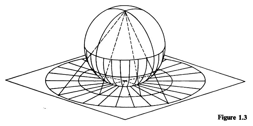
Stereographic projection is the name for a specific homeomorphism (for any ) from the n-sphere with one point removed to the Euclidean space
One thinks of both the -sphere as well as the Euclidean space as topological subspaces of in the standard way, such that they intersect in the equator of the -sphere.
For one of the corresponding poles, the stereographic projection is the map which sends a point along the line connecting it with to the equatorial plane.
If one applies stereographic projection to both possible poles of the sphere given a fixed equatorial plane, then one obtains two different homeomorphisms
The set of these two projections constitutes an atlas that exhibits the n-sphere as a topological manifold, in fact a differentiable manifold and in fact as a smooth manifold.
For and with regarded as the complex plane, then this atlas realizes the 2-sphere as a complex manifold: the Riemann sphere.
Definition
We consider the ambient canonical coordinates of , in terms of which the -sphere is the topological subspace whose underlying subset is presented as follows:
Without restriction, we may identify the given pole point in the coordinates with
hence the corresponding equatorial hyperplane with
Proposition
(standard stereographic projection)
The function which sends a point to the intersection of the line through and with the equatorial hyperplane is a homeomorphism which is given in terms of ambient coordinates by
Proof
First consider more generally the stereographic projection
of the entire ambient space minus the point onto the equatorial plane, still given by mapping a point to the unique point on the equatorial hyperplane such that the points , any sit on the same straight line.
This condition means that there exists such that
Since the only condition on is that this implies that
This equation has a unique solution for given by
and hence it follow that
Since rational functions are continuous, this function is continuous and since the topology on is the subspace topology under the canonical embedding it follows that the restriction
is itself a continuous function (because its pre-images are the restrictions of the pre-images of to ).
To see that is a bijection of the underlying sets we need to show that for every
there is a unique satisfying
-
, hence
-
;
-
;
-
-
.
The last condition uniquely fixes the in terms of the given and the remaining , as
With this, the second condition says that
hence equivalently that
By the quadratic formula the solutions of this equation are
The solution violates the first condition above, while the solution satisfies it.
Therefore we have a unique solution, given by
In particular therefore also an inverse function to the stereographic projection exists and is a rational function, hence continuous. So we have exhibited a homeomorphism as required.
Generalizations
Of course the construction in prop. does not really depend on the specific coordinates chosen there.
More generally, for any point , considered as a vector in , let be the linear subspace that is the orthogonal complement to the linear span . Then there is a homeomorphism
given by sending a point to the point in that is the intersection of the line through and with .
More generally, one may take for any affine subspace of normal to and not containing . For instance one option is to take to be the tangent space to at , embedded as a subspace of .
(see e.g. Cook-Crabb 93, section 1)
Properties
One-point compactification
The inverse map exhibits as the one-point compactification of .
Extra geometric structure
In most cases of interest one is doing geometry using stereographic projection, so the sphere and the subspace are equipped with extra structure. Taking the explicit case above (), as the formula is so simple, some structures are automatically preserved, for instance:
-
orthogonalgroup action fixing pointwise (note that these two points are sent to “” and , respectively, under )
Over other fields
Stereographic projection is a general geometric technique which can be applied to other commutative rings besides . We give a brief taste of this for the case of fields. For simplicity, we focus on conic sections, i.e., solutions sets in the projective plane to homogeneous polynomials of degree .
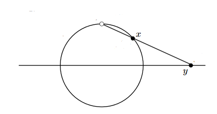
Via stereographic projection, all pointed nonsingular conic sections are isomorphic and can be identified explicitly with a projective line by means of a stereographic projection.
Geometrically, if is the chosen basepoint of and is a line not incident to , then for any other point of the unique line incident to and intersects in exactly one point, denoted . (Here is taken to be the intersection of the tangent to at with ; this can be considered the basepoint of .) In the opposite direction, to each point of , the line intersects in and (since a quadratic with one root will also have another root) another point (which might be the same as ; this happens precisely when is the tangent to at ); this gives the inverse . In this way we obtain an isomorphism of subvarieties.
Example
For the case and the rational conic , stereographic projection from the point on to the rational line defines an isomorphism of algebraic varieties . As the calculations above show, its inverse takes (for ) to .
A Pythagorean triple is a triple of integers such that , so that lies on . The isomorphism indicates that for each such point on (written as a pair of fractions in reduced form), there is a rational number (again in reduced form) so that
If we assume are coprime, and further (re)arrange the triple so that is odd and is even, one may quickly conclude from the first of this pair of equations that must have opposite parity. A little further argumentation then shows must be mutually coprime, so that in fact , and . Thus we arrive at the classical parametrization of Pythagorean triples, essentially on the basis of the geometry of stereographic projection!
Related entries
References
Textbook accounts:
- Tom Apostol, Fig. 1.3 in: Mathematical Analysis 1973 (pdf)
See also:
-
Wikipedia, Stereographic projection
-
A. L. Cook, M.C. Crabb, Fiberwise Hopf structures on sphere bundles, J. London Math. Soc. (2) 48 (1993) 365-384 (pdf)
Last revised on February 15, 2024 at 05:33:37. See the history of this page for a list of all contributions to it.