nLab fuzzy sphere

Idea

A fuzzy sphere is a variant of an n-sphere in noncommutative geometry. Often the fuzzy 2-sphere is meant by default, but there are also fuzzy spheres of higher dimension.

Definition

Fuzzy 2-sphere

For $2 \leq N \in \mathbb{N}$, the fuzzy 2-sphere of $N$ “bits” is the formal dual to the associative algebra which is the sub-algebra in the matrix algebra $Mat_{N \times N}$ generated from the elements of the $N$-dimensional complex irreducible Lie algebra representation of su(2).

We now say this more in detail:

Conventions and Normalizations

First to introduce relevant notation and to set out the proper choices of normalizations.

With $\mathfrak{su}(2)$ the Lie algebra of SU(2), whose complexification is the special linear Lie algebra sl(2) (see here)

$$\mathfrak{su}(2) \otimes_{\mathbb{R}} \mathbb{C} \;\simeq\; \mathfrak{sl}(2,\mathbb{C}) \,,$$

write

(1)$$\sigma_i \;\in\; \mathfrak{su}(2) \otimes_{\mathbb{R}} \mathbb{C} , \phantom{AAA} i \in \{1,2,3\}$$

for a choice of linear basis such that the Lie bracket takes the form

(2)$$[\sigma_i, \sigma_j] \;=\; i \underset{k}{\sum} \epsilon_{i j k} \sigma_k \,.$$

(Here $\epsilon$ is the Levi-Civita symbol, hence $\epsilon_{\sigma(1), \sigma(2)\sigma(3)} \in \{\pm 1\}$ is the signature of the permutation $\sigma \in Sym(3)$.)

Notice that the element

(3)$$\underset{i}{\sum} \sigma_i \cdot \sigma_i \;\in\; U(\mathfrak{su}(2))$$

is a Casimir element in the universal enveloping algebra.

Let then

(4)$$\rho \;\colon\; \mathfrak{su}(2) \longrightarrow Mat_{N \times N}$$

denote the complex $N$-dimensional complex irreducible Lie algebra representation of su(2) (hence of $\mathfrak{sl}(2,\mathbb{C})$).

In the discussion of angular momentum in quantum mechanics the image

(5)$$\underset{i}{\sum} \rho_i \circ \rho_i \;\in\; Mat_{N \times N}$$

of the Casimir element (3) under the representation (4) is traditionally denoted $J^2$, and the canonical linear basis for the N-dimensional representation $\rho$ (4) is then traditionally denoted $\big\{\left\vert j, m \right\rangle\big\}_{m = -j}^{m = +j}$, with

(6)$$J^2 \left\vert j,m \right\rangle \;=\; j(j+1) \phantom{--} \text{for} \phantom{-} m \in \{-j, -j+1, \cdots, j-1, j\} \,,$$

hence with

$$N(j) \,=\, 2 j + 1 \;\; \Leftrightarrow \;\; j(N) \,=\, \tfrac{1}{2}(N - 1) \,.$$

This means that the eigenvalues of (5) as a function not of the angular momentum $j$ but of the dimension $N$ of the given irreducible representation are:

(7)$$\begin{aligned} j(N)\big(j(N)+1\big) & = \phantom{+\;} (j(N))^2 + j(N) \\ & = \phantom{+\;} \tfrac{1}{4}(N-1)^2 + \tfrac{1}{2}(N-1) \\ & = \phantom{+\;} \tfrac{1}{4}N^2 - \tfrac{1}{2}N + \tfrac{1}{4} \\ & \phantom{=\;} + \tfrac{1}{2}N - \tfrac{1}{2} \\ & = \phantom{+\;} \tfrac{1}{4}N^2 - \tfrac{1}{4} \\ & = \phantom{+\;} \tfrac{1}{4} (N^2 - 1) \end{aligned}$$

Algebra of functions

Write now

(8)$$X_i \;\coloneqq\; \tfrac {2} {\sqrt{N^2-1}} \rho_N(\sigma_i)$$

for the square matrices representing the generators $\sigma_i$ (1) in the $N$-dimensional complex irrep (4), suitably normalized in view of (7).

(It is here that we need the assumption $N \geq 2$, hence excluding the complex 1-dimensional trivial irrep.)

Due to the normalization, the commutation relation (2) in this representation reads

(9)$$[X_i, X_j] \;=\; i \tfrac {2} {\sqrt{N^2-1}} \underset{k}{\sum} \epsilon_{i j k} X_k$$

and, by (7), the image of the Casimir element (3) under this representation is the identity matrix:

(10)$$\begin{aligned} R^2 & \coloneqq \underset{i}{\sum} X_i \cdot X_i \\ & = I \,. \end{aligned}$$

Equation (9) shows that in the large N limit $N \to \infty$, the algebra generated by the $X_i$ becomes commutative, and (10) says that for any $N$, the algebra generated by the $X_i$ satisfies the same relation as the smooth algebra on generators $x_i$ restricted to the actual 2-sphere of unit radius:

$$C^\infty \big( S^2 \big) \;\simeq\; SmoothAlg\big( \{x_1, x_2,x_3\}\big) \big/ \Big( \underset{i}{\sum} x_i \cdot x_i = 1 \Big)$$

Integration

With the above, the volume density of the fuzzy 2-sphere scales with $\tfrac{1}{\sqrt{N^2-1}}$

$$\begin{aligned} \tfrac{4\pi i}{3!} \epsilon^{i j k } X_i \cdot X_j \cdot X_k & = \tfrac{4\pi i}{3!} \tfrac{1}{2} \epsilon^{i j k } [X_i, X_j] \cdot X_k \\ & = \tfrac{4\pi i}{3!} \tfrac {i} {\sqrt{N^2-1}} \epsilon^{i j k } \epsilon_{i j l} X^l \cdot X_k \\ & = \tfrac{4\pi i}{3!} \tfrac {2i} {\sqrt{N^2-1}} X^k \cdot X_k \\ & = \tfrac{4\pi i}{3!} \tfrac {2i} {\sqrt{N^2-1}} \, I \\ & = - \tfrac{4\pi}{3} \tfrac {1} {\sqrt{N^2-1}} \, I \end{aligned}$$

In this vein, one defines the fuzzy refinement of the integral of functions over the 2-sphere against its canonical volume form, to be given by the matrix trace, normalized as follows

(11)$$\array{ \langle X_1, X_2, X_3\rangle &\overset{\int_{S^2_N}}{\longrightarrow}& \mathbb{C} \\ M &\mapsto& 4 \pi \tfrac{1}{ \sqrt{N^2 -1 } } tr(M) }$$

With this definition the volume of the fuzzy 2-sphere of $N$ bits comes out as

$$vol(S^2_N) \;=\; \int_{S^2_N} I \;=\; \tfrac{4 \pi}{ \sqrt{N^2 - 1 } } \underset{N}{\underbrace{tr(I)}} \;=\; 4 \pi \tfrac{ N }{ \sqrt{N^2 -1} } \,.$$

This indeed goes to the volume of the actual 2-sphere in the limit $N \to \infty$:

$$\underset{N \to \infty}{\lim} vol(S^2_N) \;=\; 4 \pi \;=\; vol(S^2) \,.$$

Properties

Shape observables as weight systems on chord diagrams

We discuss how the “shape observables” on the fuzzy 2-sphere (above) are given by single trace observables which are Lie algebra weight systems on chord diagrams (following Ramgoolam-Spence-Thomas 04, McNamara-Papageorgakis 05, see McNamara 06, Section 4 for review).

For more see at weight systems on chord diagrams in physics.

While in the commutative large N limit, all powers of the radius function are equal

$$\underset{N\to \infty}{\lim} \int_{S^2_N} R^{2 k} \;=\; 4 \pi \,;$$

for finite $N$ there is an ordering ambiguity: In fact, the number of functions on the fuzzy 2-sphere at finite $N$ that all go to the same function $R^{2k}$ in the large N limit grows rapidly with $k$.

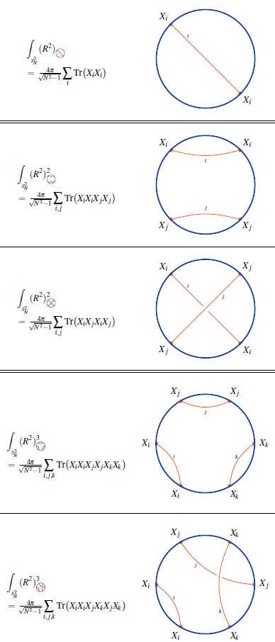
At $k = 1$ there is the single radius observable (10)

$$\int_{S^2_N} R^2 \;=\; \int_{S^2_N} \underset{i}{\sum} X_i \cdot X_i \;=\; 4 \pi \tfrac{ N }{ \sqrt{N^2 -1} }$$

At $k = 2$ there are, under the integral (11), two radius observables:

1. $\int_{S^2_N} \underset{i,j}{\sum} X_i X_i X_j X_j$

2. $\int_{S^2_N} \underset{i,j}{\sum} X_i X_j X_j X_i$

(Here we are using that under the integral/trace, a cyclic permutation of the factors in the integrand does not change the result).

Similarly for higher $k$, where the number of possible orderings increases rapidly. The combinatorics that appears here is familiar in knot theory:

Every ordering of operators, up to cyclic permutation, in the single trace observable $Tr(R^2)^n$ is encoded in a chord diagram and the value of the corresponding single trace observable is the value of the su(2)-Lie algebra weight system on this chord diagram.

from Sati-Schreiber 19c

Appearance in D-brane geometry

The fuzzy spheres appear in D-brane geometry:

1. the fuzzy funnels of Dp-D(p+2)-brane intersections have fuzzy 2-sphere slices

2. the fuzzy funnels of Dp-D(p+4)-brane intersections have fuzzy 4-sphere slices

3. the supersymmetric classical solutions of the BMN matrix model are precisely fuzzy 2-sphere configurations (BMN 02 (5.4)).

Related concepts

• fuzzy funnel

• noncommutative torus

References

General

• Ludwik Dabrowski: The Garden of Quantum Spheres, Banach Center Publications 61 (2003) 37-48 [arXiv:math/0212264, dml:282292]

Review in the context of D-brane geometry, matrix models of string theory/M-theory (BFSS matrix model, BMN matrix model, IKKT matrix model):

• Badis Ydri, Review of M(atrix)-Theory, Type IIB Matrix Model and Matrix String Theory (arXiv:1708.00734), published as: Matrix Models of String Theory, IOP 2018 (ISBN:978-0-7503-1726-9)

See also:

• David Viennot: Metrics and geodesics on fuzzy spaces [arXiv:2305.15095]

Fuzzy 2-sphere

On the fuzzy 2-sphere:

General

The fuzzy 2-sphere was introduced in:

• John Madore, The Fuzzy sphere, Class. Quant. Grav. 9 (1992) 69-88 (spire:314358)

Discussion of the spectral Riemannian geometry of the fuzzy 2-sphere:

• Francesco D'Andrea, Fedele Lizzi, Joseph Várilly, Metric Properties of the Fuzzy Sphere, Lett. Math. Phys.103 (2013), 183-205 (arXiv:1209.0108)

• Anwesha Chakraborty, Partha Nandi, Biswajit Chakraborty, A note on spectral triple with real structure on fuzzy sphere (arXiv:2111.03012)

In the context of the IKKT matrix model:

• Harold Steinacker, Non-commutative geometry and matrix models, PoS QGQGS2011 (2011) 004 (arXiv:1109.5521)

Concerning 2d CFT on the fuzzy sphere:

• Giulia Fardelli, A. Liam Fitzpatrick, Emanuel Katz: Constructing the Infrared Conformal Generators on the Fuzzy Sphere [arXiv:2409.02998]

See also:

• Wikipedia, Fuzzy sphere

Observables via weight systems on chord diagrams

Relation of Dp-D(p+2)-brane bound states (hence Yang-Mills monopoles) to su(2)-Lie algebra weight systems on chord diagrams computing radii averages of fuzzy spheres:

• Sanyaje Ramgoolam, Bill Spence, S. Thomas, Section 3.2 of: Resolving brane collapse with $1/N$ corrections in non-Abelian DBI, Nucl. Phys. B703 (2004) 236-276 (arxiv:hep-th/0405256)

• Simon McNamara, Constantinos Papageorgakis, Sanyaje Ramgoolam, Bill Spence, Appendix A of: Finite $N$ effects on the collapse of fuzzy spheres, JHEP 0605:060, 2006 (arxiv:hep-th/0512145)

• Simon McNamara, Section 4 of: Twistor Inspired Methods in Perturbative FieldTheory and Fuzzy Funnels, 2006 (spire:1351861, pdf, pdf)

• Constantinos Papageorgakis, p. 161-162 of: On matrix D-brane dynamics and fuzzy spheres, 2006 (pdf)

Fuzzy 3-sphere

The fuzzy 3-sphere was first discussed (in the context of D0-brane-systems) in

• Z. Guralnik, Sanyaje Ramgoolam, On the Polarization of Unstable D0-Branes into Non-Commutative Odd Spheres, JHEP 0102:032, 2001 (arXiv:hep-th/0101001)

Discussion in the context of M2-M5-brane bound states/E-strings:

• Anirban Basu, Jeffrey Harvey, The M2-M5 Brane System and a Generalized Nahm’s Equation, Nucl.Phys. B713 (2005) 136-150 (arXiv:hep-th/0412310)

See also:

• Samuel Kováčik, Juraj Tekel, Fuzzy Onion as a Matrix Model [arXiv:2309.00576]

Fuzzy 4-sphere

The fuzzy 4-sphere:

• Harald Grosse, Ctirad Klimcik, P. Presnajder, On Finite 4D Quantum Field Theory in Non-Commutative Geometry, Commun. Math. Phys.180:429-438, 1996 (arXiv:hep-th/9602115)

• Judith Castelino, Sangmin Lee, Washington Taylor, Longitudinal 5-branes as 4-spheres in Matrix theory, Nucl. Phys. B526:334-350, 1998 (arXiv:hep-th/9712105)

  (via D5-branes)

Fuzzy 6-sphere and higher

The fuzzy 6-sphere and higher:

• Sanjaye Ramgoolam, Section 5 of: On spherical harmonics for fuzzy spheres in diverse dimensions, Nucl. Phys. B610: 461-488, 2001 (arXiv:hep-th/0105006)

• Yusuke Kimura, On Higher Dimensional Fuzzy Spherical Branes, Nucl. Phys. B664 (2003) 512-530 (arXiv:hep-th/0301055)

• Francesco Pisacane, $O(D)$-equivariant fuzzy spheres (arXiv:2002.01901)

See also:

• Denjoe O’Connor, Brian P. Dolan, Exceptional fuzzy spaces and octonions [arXiv:2210.14754]