nLab fuzzy funnel
Context
String theory
Ingredients
Critical string models
Extended objects
Topological strings
Backgrounds
Phenomenology
Contents
Idea
The microscopic geometry of transversal Dp-D(p+2)-brane intersections and Dp-D(p+4)-brane intersections look like warped non-commutative metric cones on fuzzy spheres (namely on the spheres around the lower dimensional D-branes inside the higher dimensional D-branes). These have hence been called fuzzy funnels.
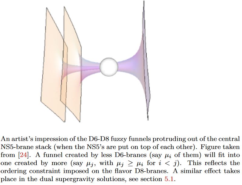
graphics grabbed from Fazzi 17, Fig. 3.14, taken in turn from Gaiotto-Tomassiello 14, Figure 5
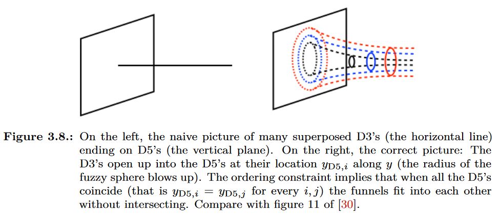
graphics grabbed from Fazzi 17
Transveral Dp-D(p+2)-brane intersections in fuzzy funnels
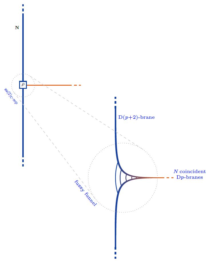
The boundary condition in the nonabelian DBI model of coincident Dp-branes describing their transversal intersection/ending with/on D(p+2)-branes is controled by Nahm's equation and thus exhibits the brane intersection-locus equivalently as:
-
a fuzzy funnel noncommutative geometry interpolating between the - and the -brane worldvolumes;
-
geometric engineering of Yang-Mills monopoles in the worldvolume-theory of the ambient -branes.
(Diaconescu 97, Constable-Myers-Fafjord 99, Hanany-Zaffaroni 99, Gaiotto-Witten 08, Section 2.4, HLPY 08, GZZ 09)
More explicitly, for the transversal distance along the stack of -branes away from the -brane, and for
the three scalar fields on the worldvolume, the boundary condition is:
as . These are Nahm's equations, solved by
where
is a Lie algebra homomorphism from su(2) to the unitary Lie algebra, and
is its complex-linear combination of values on the canonical Pauli matrix basis.
Equivalently. is an -dimensional complex Lie algebra representation of su(2). Any such is reducible as a direct sum of irreducible representations , for which there is exactly one, up to isomorphism, in each dimension :
(Here the notation follows the discussion at M2/M5-brane bound states in the BMN model, which is the M-theory lift of the present situation).
Now each irrep may be interpreted as a fuzzy 2-sphere of radius , hence as the section of a fuzzy funnel at given , whence the totality of (1) represents a system of concentric fuzzy 2-spheres/fuzzy funnels.
graphics from Sati-Schreiber 19c
Moreover, since the complexification of su(2) is the complex special linear Lie algebra (here) the solutions to the boundary conditions are also identified with finite-dimensional Lie algebra representations:
This is what many authors state, but it is not yet the full picture:
Also the worldvolume Chan-Paton gauge field component along participates in the brane intersection
its boundary condition being that
as (Constable-Myers 99, Section 3.3, Thomas-Ward 06, p. 16, Gaiotto-Witten 08, Section 3.1.1)
Together with (2) this means that the quadruple of fields constitutes a Lie algebra representation of the general linear Lie algebra
This makes little difference as far as bare Lie algebra representations are concerned, but it does make a crucial difference when these are regarded as metric Lie representations of metric Lie algebras, since admits further invariant metrics…
Properties
Single trace observables as -weight systems on chord diagrams
We discuss how the single trace observables on the fuzzy 2-sphere-sections of Dp-D(p+2) brane intersection fuzzy funnels are given by su(2)-Lie algebra weight systems on chord diagrams (following Ramgoolam-Spence-Thomas 04, McNamara-Papageorgakis 05, see McNamara 06, Section 4 for review).
For more see at weight systems on chord diagrams in physics.
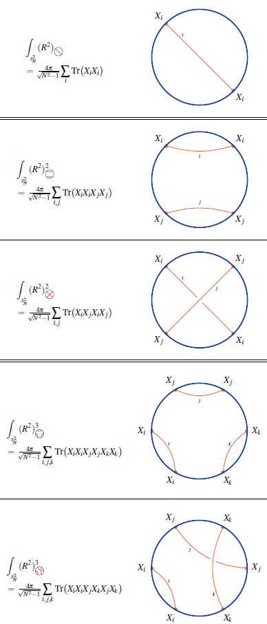
While in the commutative large N limit, all powers of the radius function on the fuzzy 2-sphere are equal
for finite there is an ordering ambiguity: In fact, the number of functions on the fuzzy 2-sphere at finite that all go to the same function in the large N limit grows rapidly with .
At there is the single radius observable (?)
At there are, under the integral (?), two radius observables:
(Here we are using that under the integral/trace, a cyclic permutation of the factors in the integrand does not change the result).
Similarly for higher , where the number of possible orderings increases rapidly. The combinatorics that appears here is familiar in knot theory:
Every ordering of operators, up to cyclic permutation, in the single trace observable is encoded in a chord diagram and the value of the corresponding single trace observable is the value of the su(2)-Lie algebra weight system on this chord diagram.
Related concepts
brane intersections/bound states/wrapped branes/polarized branes
-
D-branes and anti D-branes form bound states by tachyon condensation, thought to imply the classification of D-brane charge by K-theory
-
intersecting D-branes/fuzzy funnels:
-
Dp-D(p+6) brane bound state
References
General
- Rajsekhar Bhattacharyya, Robert de Mello Koch, Fluctuating Fuzzy Funnels, JHEP 0510 (2005) 036 (arXiv:hep-th/0508131)
For D1-D3-brane intersections
On D1-D3 brane intersections as fuzzy funnels on fuzzy 2-spheres:
-
Neil Constable, Robert Myers, Oyvind Tafjord, The Noncommutative Bion Core, Phys. Rev. D61 (2000) 106009 (arXiv:hep-th/9911136)
-
Robert Myers, Section 4 of: Nonabelian D-branes and Noncommutative Geometry, J. Math. Phys. 42: 2781-2797, 2001 (arXiv:hep-th/0106178)
-
Neil Constable, Neil Lambert, Calibrations, Monopoles and Fuzzy Funnels, Phys. Rev. D66 (2002) 065016 (arXiv:hep-th/0206243)
For D3-D5 brane intersections
On D3-D5 brane intersections as fuzzy funnels on fuzzy 2-spheres:
-
Davide Gaiotto, Edward Witten, Section 3.4.3 of: Supersymmetric Boundary Conditions in N=4 Super Yang-Mills Theory, J Stat Phys (2009) 135: 789 (arXiv:0804.2902)
-
Marco Fazzi, Section 3.2.3 of: Higher-dimensional field theories from type II supergravity (arxiv:1712.04447)
For D6-D8 brane intersections
On D6-D8 brane intersections as fuzzy funnels on fuzzy 2-spheres:
-
Davide Gaiotto, Alessandro Tomasiello, Holography for theories in six dimensions, JHEP 12 (2014) 003 (arXiv:1404.0711)
For D1-D5-brane intersections
On D1-D5 brane intersections as fuzzy funnels on fuzzy 4-spheres:
- Neil Constable, Robert Myers, Oyvind Tafjord, Non-abelian Brane Intersections, JHEP 0106:023, 2001 (arXiv:hep-th/0102080)
For D1-D7-brane intersections
On D1-D7 brane intersections as fuzzy funnels on fuzzy 6-spheres:
- Paul Cook, Robert de Mello Koch, Jeff Murugan, Non-Abelian BIonic Brane Intersections, Phys. Rev. D68:126007, 2003 (arXiv:hep-th/0306250)
Single trace observables as weight systems on chord duagrams
Relation of single trace observables on Dp-D(p+2)-brane bound states (hence Yang-Mills monopoles) to su(2)-Lie algebra weight systems on chord diagrams computing radii averages of fuzzy spheres:
-
Sanyaje Ramgoolam, Bill Spence, S. Thomas, Section 3.2 of: Resolving brane collapse with corrections in non-Abelian DBI, Nucl. Phys. B703 (2004) 236-276 (arxiv:hep-th/0405256)
-
Simon McNamara, Constantinos Papageorgakis, Sanyaje Ramgoolam, Bill Spence, Appendix A of: Finite effects on the collapse of fuzzy spheres, JHEP 0605:060, 2006 (arxiv:hep-th/0512145)
-
Simon McNamara, Section 4 of: Twistor Inspired Methods in Perturbative FieldTheory and Fuzzy Funnels, 2006 (spire:1351861, pdf, pdf)
-
Constantinos Papageorgakis, p. 161-162 of: On matrix D-brane dynamics and fuzzy spheres, 2006 (pdf)
Last revised on December 7, 2021 at 15:39:13. See the history of this page for a list of all contributions to it.