nLab functorial field theory
Context
Functorial quantum field theory
Physics
physics, mathematical physics, philosophy of physics
Surveys, textbooks and lecture notes
theory (physics), model (physics)
experiment, measurement, computable physics
-
-
-
Axiomatizations
-
Tools
-
Structural phenomena
-
Types of quantum field thories
-
Contents
- Idea
- As an axiomatization of the path integral and S-Matrix
- As the dual axiomatization to AQFT
- Global (“non-covariant”) and local (“covariant”) version
- Exposition and Introduction
- Quantum mechanics in Schrödinger picture
- Time evolution and Functors
- Entanglement and Monoidal structure
- Bra-Kets and Dual objects
- Partition functions and Monoidal string diagrams
- Path integral quantization of 1d Gauge theory
- Gauge transformation and Groupoids
- Trajectories of fields and Correspondences of groupoids
- Action functionals and Slice groupoids
- Quantum mechanics with interactions and Feynman diagrams
- Spectral triples and Graph representations
- Feynman diagram in worldline formalism and Monoidal string diagrams
- Quantum topological string
- Global 2d TQFT and Frobenius algebra
- Cohomological 2d TQFT and Calabi-Yau -algebras
- Local 2d TQFT and 2-Modules
- General local TQFT
- 3d TQFT
- Related concepts
- References
- Terminology
- Formalization of sewing and locality in terms of functoriality
- Relation between algebraic and functorial field theory
- Non-topological FQFTs (especially conformal)
- Extended (multi-tiered) FQFT
- (extended) FQFT from background fields: -models
- Super QFT
- homological 2d FQFT (and TCFT)
- CFT as functorial field theory
- The , SCFT as an extended functorial field theory
Idea
Functorial quantum field theory or FQFT for short, is one of the two approaches of providing a precise mathematical formulation of and of axiomatizing quantum field theory. FQFT formalizes the Schrödinger picture of quantum mechanics (generalized to quantum field theory) where spaces of quantum states are assigned to space and where linear maps are assigned to trajectories/spacetimes interpolating between these spaces.
As an axiomatization of the path integral and S-Matrix
The axioms of FQFT may be understood as formulating the basic properties that the path integral or S-matrix invoked in physics ought to satisfy, if they had been given a precise definition.
Much work in quantum field theory is based on arguments invoking the concept of the path integral. While in the physics literature this is usually not a well defined object, it is generally assumed to satisfy a handful of properties, notably the sewing laws. These say, roughly, that the path integral over a domain which decomposes into subdomains and is the same as the path integral over composed with that over .
Accordingly it is the S-matrix that is manifestly incarnated in the Atiyah-Segal picture of functorial QFT:
Here a quantum field theory is given by a monoidal functor
from a suitable monoidal category of cobordisms to a suitable monoidal category of vector spaces.
-
To a codimension-1 slice of space this assigns a vector space – the (Hilbert) space of quantum states over ;
-
to a spacetime/worldvolume manifold with boundaries one assigns the quantum propagator which is the linear map that takes incoming states to outgoing states via propagation along the spacetime/worldvolume . This is alternatively known as the the scattering amplitude or S-matrix for propagation from to along a process of shape .
Now for genuine topological field theories all spaces of quantum states are finite dimensional and hence we can equivalently consider the dual vector space (using that finite dimensional vector spaces form a compact closed category). Doing so the propagator map
equivalently becomes a linear map of the form
Notice that such a linear map from the canonical 1-dimensional complex vector space to some other vector space is equivalently just a choice of element in that vector space. It is in this sense that is equivalently a vector in .
In this form in physics the propagator is usually called the correlator or n-point function .
The axioms of (Segal 04) for FQFT (2d CFT in this case) were originally explicitly about the propagators/S-matrices, while (Atiyah 88) formulated it in terms of the correlators this way. Both perspectives go over into each other under duality as above.
Notice that this kind of discussion is not restricted to topological field theory. For instance already plain quantum mechanics is usefully formulated this way, that’s the point of finite quantum mechanics in terms of dagger-compact categories.
As the dual axiomatization to AQFT
Historically older is the proposal for axiomatizing QFT that is known as AQFT, short for algebraic quantum field theory. This formalizes the Heisenberg picture of quantum mechanics, as do modern variants such as factorization algebras. Here the basic assignment is that of algebras of observables to regions of spacetime.
In principle AQFT and FQFT should be two sides of the same medal, and in special cases this has been made precise (see for instance at topological chiral homology) but generally, much as the formulation of FQFT and AQFT themselves remains in progress, so does their precise relation.
duality between algebra and geometry
in physics:
Global (“non-covariant”) and local (“covariant”) version
Functorial QFT in any dimension was originally formulated (Atiyah 88, Segal 04) as a 1-functor on a 1-category of cobordisms. In this formulation there is a space of quantum states assigned to every global spatial slice of spacetime/worldvolume, which is then propagated in time/along a parameter. In physics jargon this corresponds to “non-covariant” quantization, in that the slicing of spacetime/worldvolume into space and time components breaks general covariance which is the hallmark specifically of the topological quantum field theories to which the methods of FQFT apply most immediately.
A local (“extended”, “multi-tiered”) refinement of this is naturally given by passing from 1-functors to (∞,n)-functors on (∞,n)-categories of cobordisms. This formulation was vaguely suggested in (Baez-Dolan 95) (“cobordism hypothesis”) and formalized in (Lurie 09). It captures what in physics jargon would be called “covariant” quantum field theory, in that the “localization down to the point” means that the formalism knows how to glue/propagate in spatial directions just as in time directions, in fact that no such distinction is retained.
Exposition and Introduction
under construction
We give here motivation for, introduction to and an exposition of the ideas of local (extended) functorial field theory.
We start in
by showing how all the basic category-theoretic ideas are already right beneath the surface of the traditional textbook discussion of quantum mechanics. Following that in
we show for the simple case of 1-dimensional finite gauge theory how also path integral quantization of prequantum (classical) data is naturally organized by monoidal category theory with first bits of homotopy theory showing up (that will play a more paramount role as one goes up in dimension).
Then in
this becomes all the more pronounced when one considers quantum mechanics with interaction as in the worldline formalism and hence when one considers Feynman diagrams as diagrams of interactions of particles.
This 1-dimensional functorial description worldline quantum mechanics has an evident generalization to a worldsheet formulation of 2d topological field theory. This original 1-functorial TQFT axiomatics due to Atiyah and Segal we review in
However, this “naive” generalization is not quite refined enough. Physically one sees this from the fact that the topological string A-model/B-model, which is the archetype of a 2d TQFT in physics, is not actually an instance of the Atiyah-Segal axiomatics. Mathematically one sees it from the fact that the 1-category theoretic formulation of 2d boundary field theory is clearly lacking a “categorical dimension” in order to be satisfactory.
The correct refinement of 2d TQFT to a cohomological field theory or “TCFT” with coefficients not just in vector spaces but in chain complexes of vector spaces we then consider in
This gives a natural conceptual home to the derived categories of D-branes famous from homological mirror symmetry. But it is still not quite the fully general functorial formalization of quantum field theory.
To get a feeling for what is missing, we next consider 3d TQFT
This finally is enough information to naturally motivate the full formulation of the cobordism hypothesis in symmetric monoidal (infinity,n)-category theory in
Quantum mechanics in Schrödinger picture
This section introduces the observation that the basic structures in quantum mechanics are accurately reflected in symmetric monoidal category theory, by explaining the following dictionary:
Time evolution and Functors
The basic idea of quantum mechanics in the “Schrödinger picture” is to describe a quantum mechanical system (such as an electron in the electromagnetic field of a proton) by
-
assigning to each time a vector space (Hilbert space) to be thought of as the space of quantum states (of pure states, that is) of the system at that time;
-
assigning to each pair of times a linear operator (unitary operator) to be thought of as encoding the time evolution of quantum states
such that
-
this assignment is local in time in that for all one has
In basic quantum mechanics one also demands that
(While this looks like the most innocent condition, this has technical subtleties for genuine quantum field theory, to deal with which however there exist established tools.)
The locality condition intuitively says that “all global effects arise by integrating up local effects”. Indeed, when assuming in addition that depends smoothly on the time arguments, then the locality condition is equivalent to (see at parallel transport) the existence of a Hamiltonian , a self-adjoint operator depending smoothly on , such that time evolution is given by the Dyson formula
(Here the notation on the right denotes the “path ordered exponential”, see at parallel transport.) In the special case that the Hamiltonian is time-independent, , then this reduces to
This is the way that quantum mechanical time evolution is traditionally introduced in the textbooks.
But the equivalent formulation above in terms of locality of is noteworthy. The condition of locality here is precisely what in mathematics is called functoriality: the condition that a system of homomorphisms (here: linear/unitary operator) depends on another system of “directed data” (here: the time intervals ) such that composition is respected.
More specifically, one says that the collection Vect (or Hilb) of vector spaces (Hilbert spaces) forms a category whose objects are vector space and whose morphisms are linear maps ; where the point is that these morphisms may be associatively composed whenever their codomain/domain matches:
Similarly, there is a category whose objects are instants of time , whose morphisms are time intervals , and whose composition operation is concatenation of time intervals
Given two categories like this, then a function that takes morphisms of one to morphisms of the other such that composition is respected is called a functor.
In this language, the above locality condition of quantum mechanics says that quantum time evolution is a functor
that takes
If this looks like a trivial reformulation of textbook material, then this is because it is a trivial reformulation of textbook material. But introducing such category-theoretic language for making the locality principle in quantum mechanics fully manifest turns out to be rather useful for capturing the full locality of local quantum field theory, which is not in the traditional textbooks. This we come to below.
| physics | category theory |
|---|---|
| locality of time evolution | functor |
Entanglement and Monoidal structure
Besides the time evolution, there is the theory of composite systems.
Given two quantum mechanical systems (e.g. of two electrons orbiting the same atomic nucleus), with spaces of quantum states (pure states) and , respectively, then the space of quantum states of the compound system is given by the tensor product of vector spaces (of Hilbert spaces)
This should be compared with the way compound systems are formed in classical mechanics: for and the configuration spaces/phase spaces of two classical mechanical systems, then the configuration space/phase space of their compound is the Cartesian product .
These Cartesian products and tensor products extend to morphisms. If is a linear operator acting on the first system and is one acting on the second system, then there is a tensor product morphism
Hence (Cartesian or non-cartesian) tensor products are something like product operations on sets, but on whole categories. Since binary associative product operations on sets are sometimes called monoids, one says that the category Vect of vector spaces when equipped with the tensor product of vector spaces is a monoidal category.
Similarly, the categories Diff or Set, of smooth manifolds or just bare sets, carry a monoidal structure given simply by the Cartesian product of sets. This is called a cartesian monoidal structure.
The characteristic property of Cartesian products is that elements of these are equivalently pairs of elements in and , respectively. This reflects in turn the characteristic property of compound classical mechanical systems: a state of these is simply a pair of states of the two subsystems.
The tensor product on Vect however is not Cartesian: an element in need not be of the form , for . Instead, in general it is a sum of such elements
In terms of physics such non-cartesian vectors are quantum states that exhibit entanglement. This hallmark property of quantum mechanics is hence accurately reflected by the abstract property of being a non-cartesian monoidal category.
| physics | category theory |
|---|---|
| entanglement | non-cartesian monoidal category of spaces of states |
For more exposition of this point see (Baez 04).
Bra-Kets and Dual objects
Consider now for simplicity of notation an application in quantum computing/quantum information theory, where the spaces of states involved are finite dimensional vector spaces (spaces of qubits), such as for instance in the topological sector of the quantum Hall system.
Then for every space of states there is the dual vector space . In physics notation the states in are the kets , while those of are the “bra”s .
| physics | category theory |
|---|---|
| bra/ket | dual objects |
Essentially all of quantum information theory has a slick reformulation in terms of category theory for symmetric monoidal category with dual objects. More on this is at finite quantum mechanics in terms of dagger-compact categories.
While the introduction of bra-ket notation by Paul Dirac was (while just notation) already quite useful for thinking about the subject, the language of monoidal categories in fact reflects the actual physical processes involved even better.
For instance, in quantum mechanics textbooks one often sees the following manipulation of symbols for expressing a trace in terms of a sum over basis elements
This “rotation” operation where symbols are cyclically permuted reflects the fact that indeed traces as in partition functions reflect actual physical circular processes.
In “string diagram”-notation of monoidal category-theory this is reflected as follows. The unit map
is depicted as
and the counit map
as
Partition functions and Monoidal string diagrams
Given a Hamiltonian , the partition function of the quantum mechanical system is the trace
In bra-ket notation this is
In terms of monoidal category-theoretic notation (string diagrams) this same expression reads as follows
This is striking, because this picture is an accurate reflection of the physical process that the partition function describes, for the partition function is the correlator of a particle with a closed circular worldline.
In fact, the monoidal category theoretic string diagram-notation is essentially the Feynman diagram-notation. This we turn to below.
For a 1-dimensional TQFT the Hamiltonian above vanishes. (Or maybe more interestingly: for supersymmetric quantum mechanics the Hamiltonian may not vanish, but in the super trace in the partition function all non-zero energy eigenmodes cancel out by supersymmetry, and only the topological part is left after all.)
In this case the partition function reduces to
which is just the trace on .
To reflect this in the functorial notation from above, notice that also the category from above is naturally a monoidal category if we take its objects to consist not just of single points, but of arbitrary collections of points, and to have its morphisms consist of all 1-dimensional cobordisms. Then a monoidal structure is given by disjoint union.
A 1d TQFT with values in vector spaces is then a strong monoidal functor
Other processes that such a 1d TQFT encodes include
In this way a 1d TQFT is entirely encoded in the operation that exhibit a finite dimensional vector space as a dualizable object.
1d TQFT with coefficients in Vect
finite dimensional vector spaces
This is the simplest incarnation of the statement that for higher dimensional extended TQFT becomes the cobordism hypothesis. We come to this below.
Path integral quantization of 1d Gauge theory
The path integral tends to be as suggestive in quantum field theory as it is invoked ubiquitously, and FQFT may be understood as being precisely the axiomatics that a would-be path integral ought to satisfy, thereby decoupling its construction as a suitably regularized integral from its operational definition as yielding a consistent S-matrix for the QFT.
We discuss now the simplest non-trivial example of a path integral quantization, namely for 1-dimensional finite gauge theory, the 1-dimensional Dijkgraaf-Witten model. This has the two-fold purpose of
-
indicating how not just the final quantum theory but also its prequantum data is naturally organized by monoidal category theory;
-
motivating and introducing elements of homotopy theory which become crucial for the understanding of FQFT as one moves up in dimension.
A more detailed version of this section is at Local prequantum field theory – id Dijkgraaf-Witten theory.
Gauge transformation and Groupoids
The following is a quick review of basics of groupoids and their homotopy theory (homotopy 1-type-theory), geared towards the constructions and facts needed for 1-dimensional Dijkgraaf-Witten theory.
Definition
-
a pair of sets (the set of objects) and (the set of morphisms)
-
equipped with functions
where the fiber product on the left is that over ,
such that
-
takes values in endomorphisms;
-
defines a partial composition operation which is associative and unital for the identities; in particular
and ;
-
every morphism has an inverse under this composition.
Remark
This data is visualized as follows. The set of morphisms is
and the set of pairs of composable morphisms is
The functions are those which send, respectively, these triangular diagrams to the left morphism, or the right morphism, or the bottom morphism.
Example
For a set, it becomes a groupoid by taking to be the set of objects and adding only precisely the identity morphism from each object to itself
Example
For a group, its delooping groupoid has
-
;
-
.
For and two groups, group homomorphisms are in natural bijection with groupoid homomorphisms
In particular a group character is equivalently a groupoid homomorphism
Here, for the time being, all groups are discrete groups. Since the circle group also has a standard structure of a Lie group, and since later for the discussion of Chern-Simons type theories this will be relevant, we will write from now on
to mean explicitly the discrete group underlying the circle group. (Here “” denotes the “flat modality”.)
Example
For a set, a discrete group and an action of on (a permutation representation), the action groupoid or homotopy quotient of by is the groupoid
with composition induced by the product in . Hence this is the groupoid whose objects are the elements of , and where morphisms are of the form
for , .
As an important special case we have:
Example
For a discrete group and the trivial action of on the point (the singleton set), the coresponding action groupoid according to def. is the delooping groupoid of according to def. :
Another canonical action is the action of on itself by right multiplication. The corresponding action groupoid we write
The constant map induces a canonical morphism
This is known as the -universal principal bundle. See below in for more on this.
Example
For a topological space, its fundamental groupoid is
- points in ;
- continuous paths in modulo homotopy that leaves the endpoints fixed.
Example
For any groupoid, there is the path space groupoid with
-
;
-
commuting squares in =
This comes with two canonical homomorphisms
which are given by endpoint evaluation, hence which send such a commuting square to either its top or its bottom hirizontal component.
Definition
For two morphisms between groupoids, a homotopy (a natural transformation) is a homomorphism of the form (with codomain the path space object of as in example ) such that it fits into the diagram as depicted here on the right:
Definition (Notation)
Here and in the following, the convention is that we write
-
(with the subscript decoration) when we regard groupoids with just homomorphisms (functors) between them,
-
(without the subscript decoration) when we regard groupoids with homomorphisms (functors) between them and homotopies (natural transformations) between these
The unbulleted version of groupoids are also called homotopy 1-types (or often just their homotopy-equivalence classes are called this way.) Below we generalize this to arbitrary homotopy types (def. ).
Definition
A (homotopy-) equivalence of groupoids is a morphism which has a left and right inverse up to homotopy.
Example
The map
which picks any point and sends to the loop based at that point which winds around times, is an equivalence of groupoids.
Proposition
Assuming the axiom of choice in the ambient set theory, every groupoid is equivalent to a disjoint union of delooping groupoids, example – a skeleton.
Remark
The statement of prop. becomes false as when we pass to groupoids that are equipped with geometric structure. This is the reason why for discrete geometry all Chern-Simons-type field theories (namely Dijkgraaf-Witten theory-type theories) fundamentally involve just groups (and higher groups), while for nontrivial geometry there are genuine groupoid theories, for instance the AKSZ sigma-models. But even so, Dijkgraaf-Witten theory is usefully discussed in terms of groupoid technology, in particular since the choice of equivalence in prop. is not canonical.
Definition
Given two morphisms of groupoids their homotopy fiber product
hence the ordinary iterated fiber product over the path space groupoid, as indicated.
Remark
An ordinary fiber product of groupoids is given simply by the fiber product of the underlying sets of objects and morphisms:
Example
For a groupoid, a group and a map into its delooping, the pullback of the -universal principal bundle of example is equivalently the homotopy fiber product of with the point over :
Namely both squares in the following diagram are pullback squares
(This is the first example of the more general phenomenon of universal principal infinity-bundles.)
Example
For a groupoid and a point in it, we call
the loop space groupoid of .
For a group and its delooping groupoid from example , we have
Hence is the loop space object of its own delooping, as it should be.
Proof
We are to compute the ordinary limiting cone in
In the middle we have the groupoid whose objects are elements of and whose morphisms starting at some element are labeled by pairs of elements and end at . Using remark the limiting cone is seen to precisely pick those morphisms in such that these two elements are constant on the neutral element , hence it produces just the elements of regarded as a groupoid with only identity morphisms, as in example .
Proposition
The free loop space object is
Proof
Notice that . Therefore the path space object has
-
objects are pairs of morphisms in ;
-
morphisms are commuting squares of such.
Now the fiber product in def. picks in there those pairs of morphisms for which both start at the same object, and both end at the same object. Therefore is the groupoid whose
-
objects are diagrams in of the form
-
morphism are cylinder-diagrams over these.
One finds along the lines of example that this is equivalent to maps from into and homotopies between these.
Remark
Even though all these models of the circle are equivalent, below the special appearance of the circle in the proof of prop. as the combination of two semi-circles will be important for the following proofs. As we see in a moment, this is the natural way in which the circle appears as the composition of an evaluation map with a coevaluation map.
Example
For a discrete group, the free loop space object of its delooping is , the action groupoid, def. , of the adjoint action of on itself:
Example
For an abelian group such as we have
Example
Let be a group homomorphism, hence a group character. By example this has a delooping to a groupoid homomorphism
Under the free loop space object construction this becomes
hence
So by postcomposing with the projection on the first factor we recover from the general homotopy theory of groupoids the statement that a group character is a class function on conjugacy classes:
Trajectories of fields and Correspondences of groupoids
With some basic homotopy theory of groupoids in hand, we can now talk about trajectories in finite gauge theories, namely about spans/correspondences of groupoids and their composition. These correspondences of groupoids encode trajectories/histories of field configurations.
Namely consider a groupoid to be called Grpd, to be thought of as the moduli space of fields in some field theory, or equivalently and specifically as the target space of a sigma-model field theory. This just means that for any manifold thought of as spacetime or worldvolume, the space of fields of the field theory on is the mapping stack (internal hom) from into , which means here for DW theory that it is the mapping groupoid, def. , out of the fundamental groupoid, def. , of :
We think of the objects of the groupoid as being the fields themselves, and of the morphisms as being the gauge transformations between them.
The example to be of interest in a moment is that where is a delooping groupoid as in def. , in which case the fields are equivalently flat principal connections. In fact in the discrete and 1-dimensional case currently considered this is essentially the only example, due to prop. , but for the general idea and for the more general cases considered further below, it is useful to have the notation allude to more general moduli spaces .
The simple but crucial observation that shows why spans/correspondences of groupoids show up in prequantum field theory is the following.
Example
If is a cobordism, hence a manifold with boundary with incoming boundary component and outgoing boundary components , then the resulting cospan of manifolds
is sent under the operation of mapping into the moduli space of fields
to a span of groupoids
Here the left and right homomorphisms are those which take a field configuration on and restrict it to the incoming and to the outgoing field configuration, respectively. (And this being a homomorphism of groupoids means that everything respects the gauge symmetry on the fields.) Hence if is thought of as the spaces of incoming and outgoing field configurations, respectively, then is to be interpreted as the space of trajectories (sometimes: histories) of field cofigurations over spacetimes/worldvolumes of shape .
This should make it plausible that specifying the field content of a 1-dimensional discrete gauge field theory is a functorial assignment
from a category of cobordisms of dimension one into a category of such spans of groupoids. It sends points to spaces of field configurations on the point and 1-dimensional manifolds such as the circle to spaces of trajectories of field configurations on them.
Moreover, for a local field theory it should be true that the field configurations on the circle, say, are determined from gluing the field configurations on any decomposition of the circle, notably a decomposition into two semi-circles. But since we are dealing with a topological field theory, its field configurations on a contractible interval such as the semicircle will be equivalent to the field configurations on the point itself.
The way that the fields on higher spheres in a topological field theory are induced from the fields on the point is by an analog of traces for spaces of fields, and higher traces of such correspondences (the “span trace”). This is because by the cobordism theorem, the field configurations on, notably, the n-sphere are given by the -fold span trace of the field configurations on the point, the trace of the traces of the … of the 1-trace. This is because for instance the 1-sphere, hence the circle is, regarded as a 1-dimensional cobordism itself pretty much manifestly a trace on the point in the string diagram formulation of traces.
Here is the point with its positive orientation, and is its dual object in the category of cobordisms, the point with the reverse orientation. Since, by this picture, the construction that produces the circle from the point is one that involves only the coevaluation map and evaluation map on the point regarded as a dualizable object, a topological field theory , since it respects all this structure, takes the circle to precisely the same kind of diagram, but now in , where it becomes instead the span trace on the space over the point. This we discuss now.
Before talking about correspondences of groupoids, we need to organize the groupoids themselves a bit more.
Definition
A (2,1)-category is
-
a collection – the “collection of objects”;
-
for each tuple a groupoid – the hom-groupoid from to ;
-
for each triple a groupoid homomorphism (functor)
called composition or horizontal composition for emphasis;
-
for each quadruple a homotopy – the associator –
(…) and similarly a unitality homotopy (…)
such that for each quintuple the associators satisfy the pentagon identity.
The objects of the hom-groupoid we call the 1-morphisms from to , indicated by , and the morphisms in we call the 2-morphisms of , indicated by
If all associators can and are chosen to be the identity then this is called a strict (2,1)-category.
Definition/Example
Write Grpd for the strict (2,1)-category, def. , whose
-
1-morphisms are functors ;
-
2-morphisms are homotopies between these.
Definition/Example
Write for the (2,1)-category whose
-
1-morphisms are spans/correspondences of functors, hence
-
2-morphisms are diagrams in Grpd of the form
-
composition is given by forming the homotopy fiber product, def. , of the two adjacent homomorphisms of two spans, hence for two spans
and
their composite is the span which is the outer part of the diagram
Definition
There is the structure of a symmetric monoidal (2,1)-category on by degreewise Cartesian product in Grpd.
Definition
An object of a symmetric monoidal (2,1)-category is fully dualizable if there exists
-
another object , to be called the dual object;
-
a 1-morphism , to be called the evaluation map;
-
a 1-morphism , to be called the coevaluation map;
-
and
and
(the saddle?)
and
(the co-saddle)
such that these exhibit an adjunction and are themselves adjoint (…).
Definition
Given a symmetric monoidal (2,1)-category , and a fully dualizable object and a 1-morphism , the trace of is the composition
Proposition
Every groupoid is a dualizable object in , and in fact is self-dual.
The evaluation map , hence the possible image of a symmetric monoidal functor of a cobordism of the form
is given by the span
and the coevaluation map by the reverse span.
For any object, the trace (“span trace”) of the identity on it, hence the image of
is its free loop space object, prop. :
The second order covaluation map on the span trace of the identity is
Proof
By prop. the trace of the identity is given by the composite span
Along these lines one checks the required zig-zag identities.
Action functionals and Slice groupoids
We have now assembled all the ingredients need in order to formally regard a group character on a discrete group as a local action functional of a prequantum field theory, hence as a fully dualizable object
in a (2,1)-category of correspondences of groupoids as in def. , but equipped with maps and homotopies between maps to the coefficient over . This is described in def. below. Before stating this, we recall for the 1-dimensional case the general story of def. .
Example
Given a discrete groupoid , functions
are in natural bijection with homotopies of the form
where the function corresponding to this homotopy is that given by the unique factorization through the homotopy fiber product (example ) as shown on the right of
This means that if we have an action functional on a space of trajectories, and if these trajectories are given by spans/correspondences of groupoids as discussed above, then the action functional is naturally expressed as the homotopy filling a completion of the span to a square diagram over . Therefore we cosider the following.
Definition
Write for the (2,1)-category whose
-
2-morphisms are morphism of spans compatible with the maps to in the evident way.
The operation of composition is as in , def. on the upper part of these diagrams, naturally extended to the whole diagrams by composition of the homotopies filling the squares that appear.
Proposition
carries the structure of a symmetric monoidal (2,1)-category where the tensor product is given by
Remark
There is an evident forgetful (2,1)-functor
which forgets the maps to and the homotopies between them. This is a monoidal (2,1)-functor.
As generalization of prop. we now have the following:
In conclusion we may now compute what the 1-dimensional prequantum field theory defined by a group character regarded as a local action functional assigns to the circle.
Theorem
The prequantum field theory defined by a group character
assigns to the circle the trace of the identity on this object, which under the identifications of example , example , and example is the group character itself:
Here the action functional on the right sends a field configuration to its value under the group character.
Remark
It follows that in a discussion of quantization the path integral for the partition function of 1d DW theory is given by the Schur integral over the group character .
In conclusion, 1-dimensional Dijkgraaf-Witten theory as a prequantum field theory comes down to be essentially a geometric interpretation of what group characters are and do. One may regard this as a simple example of geometric representation theory. Simple as this example is, it contains in it the seeds of many of the interesting aspects of richer prequantum field theories.
Quantum mechanics with interactions and Feynman diagrams
We saw above that symmetric monoidal category theory naturally captures all the key aspects of basic quantum mechanics.
This becomes all the more pronounced when one considers quantum mechanics with interaction as in the worldline formalism and hence when one considers Feynman diagrams as diagrams of interactions of particles.
Spectral triples and Graph representations
Let be the cobordism category of Feynman graphs for the superparticle with a single type of interaction along the lines of (1,1)-dimensional Euclidean field theories and K-theory. So its morphisms are generated from -dimensional super-Riemannian manifolds (i.e. super-intervals) and from a single interaction vertex
subject to the obvious associativity condition.
Then a spectral triple is the data encoding a sufficiently nice smooth functor
to the category of super vector spaces.
Here
-
is the even part of the super vector space assigned by the functor to the point, equipped with the structure of a algebra whose product is given by the image of the interaction vertex
-
is some completion of to a super Hilbert space
-
and is an odd self-adjoint operator on , which gives the value of the functor on the super-interval by
So this is the quantum mechanics of a superparticle. In the simplest case this comes from a spinor particle propagating on a spin structure Riemannian manifold in which case
-
is the space of square integrable spinor sections;
-
is the Dirac operator
-
is the space of smooth functions on .
One point of a spectral triple is to take the view of world-line quantum mechanics as basic and characterize the spin Riemannian geometry of entirely by this algebraic data. In particular the Riemannian metric on is encoded in the operator spectrum of , which is where the notion “spectral triple” gets its name from.
Then with all the ordinary geoemtry re-encoded algebraically this way, in terms of the 1-dimensional quantum field theory that probes this geometry, one can then use the same formulas to interpret spectral triple geometrically that do not come from an ordinary geometry as in the above example.
Feynman diagram in worldline formalism and Monoidal string diagrams
Quantum topological string
Global 2d TQFT and Frobenius algebra
In view of the above discussion of “topological quantum mechanics”, i.e. of 1-dimensional TQFT, it is immediate to pass to a higher dimensional field theory by using categories of cobordisms of higher dimension and consider strong monoidal functors
for instance 1-dimensional cobordisms with boundary describe a kind 2d TQFT with boundary field theory.
As almost immediate from these picture, such 2d TQFTs are equivalent to Frobenius algebras .
In terms of physics: is the space of states of a topological open string and the algebra and coalgebra structure on it encodes its 3-point functions.
More generally open and closed strings
Now is equivalent to a pair consisting of a Frobenius algebra and a commutative Frobenius algebra and a homomorphism to the center of
(Moore-Segal Lazaroiu 00, see also Lauda-Pfeiffer 05).
In physics speak is the space of states for the topological closed string.
Or rather, it is some topological string model, but not the one originally obtained by topological twist from the 2d (2,0)-superconformal QFT which is commonly what is understood as the “topological string” in string theory (A-model/B-model).
Cohomological 2d TQFT and Calabi-Yau -algebras
Curiously, the above does not capture the original motivating examples for 2d TQFT that came from physics, namely it does not capture the “cohomological quantum field theory” due to Edward Witten, such as the topological string in its incarnation as the A-model and B-model and the Landau-Ginzburg model.
-
Witten cohomological field theory: space of quantum states is chain complex, physical quantum states are chain homology
-
Kontsevich: homological mirror symmetry is equivalence of A-∞ categories
-
Aspinwall, Douglas et al: the derived categories here are those of topological A-branes (A-branes/B-branes)
Hence need to regard A-model/B-model open topological string as having a chain complex of vector spaces. Under string composition this yields not just an associative algebra with trace but an A-∞ algebra with suitable trace.
Examples come from twisting the 2d (2,0)-CFT induced from a Calabi-Yau manifold, hence one speaks of “Calabi-Yau A-∞ algebra”.
remember space of diffeomorphism
- Getzler, Segal: “TCFT”
classification by (Costello 04) sums it up:
Calabi-Yau A-∞ category is equivalent to non-compact open topological string with coefficients in . The objects of the category are the D-branes, hom-spaces are the spaces of quantum states of open strings stretching between these. The closed string bulk field theory sector is given by forming Hochschild homology. Given a Calabi-Yau manifold, then the A-∞ category refinement (see at enhanced triangulated category) of its derived category of coherent sheaves is an example.
Local 2d TQFT and 2-Modules
Given an associative algebra then its category of modules behaves much like a higher analog of a module/vector space.
Given an - bimodule then behaves like a higher dimensional linear operator.
This is the Eilenberg-Watts theorem.
Hence we speak of a 2-module.
Notice that every algebra is canonically an --bimodule. This way we see that the above construction naturally localizes
| cohomological QFT | local QFT | |
|---|---|---|
| open string | open string algebra | open string bimodule |
| point | 2-module |
Hence we regard D-Brane? states as quantum 2-states.
We motivate this further below. First to record the classification results:
| 2d TQFT (“TCFT”) | coefficients | algebra structure on space of quantum states | |
|---|---|---|---|
| open topological string | Vect | Frobenius algebra | folklore+(Abrams 96) |
| open topological string with closed string bulk theory | Vect | Frobenius algebra with trace map and Cardy condition | (Lazaroiu 00, Moore-Segal 02) |
| non-compact open topological string | Ch(Vect) | Calabi-Yau A-∞ algebra | (Kontsevich 95, Costello 04) |
| non-compact open topological string with various D-branes | Ch(Vect) | Calabi-Yau A-∞ category | “ |
| non-compact open topological string with various D-branes and with closed string bulk sector | Ch(Vect) | Calabi-Yau A-∞ category with Hochschild cohomology | “ |
| local closed topological string | 2Mod(Vect) over field | separable symmetric Frobenius algebras | (SchommerPries 11) |
| non-compact local closed topological string | 2Mod(Ch(Vect)) | Calabi-Yau A-∞ algebra | (Lurie 09, section 4.2) |
| non-compact local closed topological string | 2Mod for a symmetric monoidal (∞,1)-category | Calabi-Yau object in | (Lurie 09, section 4.2) |
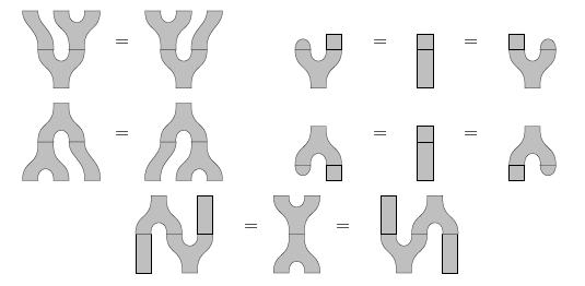
Here the trace operation in the CY conditions corresponds to the cobordism which is the “disappearance of a circle”.
One may view this as exhibiting “higher order duality”: where the semi-circles exhibits as a dual object to , this disappearance of a circle exhibits the upper semi-circle as adjoint to the lower semicircle.
(…)
General local TQFT
Covariant quantization and Directed homotopy types
One way to understand from the point of view of physics why the 1-functorial description of 2d CFT and 2d TQFT above is unsatisfactory is that it breaks what is known as “covariance” in physics, in the sense of “general covariance” (reflected also in the term “covariant phase space”): implicit in the concept of a category of cobordisms is a splitting of a spacetimes/worldvolumes into spatial slices (the objects) of the category and trajectories between these.
The standard Lagrangian-data (“prequantum field theory”) from which topological quantum field theories are supposed to arise under quantization do not enforce such a splitting as indeed they are generally covariant. Accordingly, a local Lagrangian should, after quantization, give rise to a local quantum field theory that is still “generally covariant” in that it does not require or depend on such a splitting. In physics this plays a crucial role for instance in considerations related to quantum gravity.
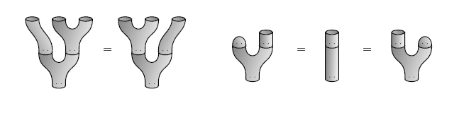
We saw above how 1-dimensional (prequantum) field theory is encoded by correspondences of groupoids. For instance the process of a particle and its antiparticle appearing out of the vacuum is given by
and the reverse process of them disappearing is given by
A particle tracing out a circle is equivalently the composition (via homotopy fiber product) of these two process.
Then we saw above for 2d TQFT that in higher dimensional general such a circle in turn may appear
and disappear
The 2-dimensional composition of such processes, again by homotopy fiber product yields values on all higher spheres
and in fact all homotopy types of smooth manifolds. For instance the trinion process is represented by this correspondence-of-correspondences:
To describe local propagation in higher dimensional field theory this way, evidently we need a higher dimensional calculus that deals both with the homotopy theory (gauge theory) involves as well as with the directionality of these processes.
We already saw the first hint of how this works: groupoids above appeared in two different guises, on the one hand as homotopy 1-types, on the other as special kinds of categories with directed morphisms.
Now homotopy 1-types have a classical generalization to general homotopy types, traditionally taken to be represented by topological spaces regarded up to weak homotopy equivalence.
A crucial fact is that one may pair this full homotopy-theoretic aspect with the category-theoretic aspect to get ∞-categories
-fold -categories (∞,n)-categories
k-morphisms for all , such that for they are invertible
in particular
-
(∞,n)-category of (∞,n)-modules?
-Spaces of states and the Cobordism hypothesis
These (∞,n)-categories are symmetric monoidal (∞,n)-categories in the same way that their 1-categorical shadows are, only that everything is lifted up to homotopy.
hence one may consider
The classification theory of these, the cobordism theorem says roughly that such local topological field theories assign fully dualizable objects to the point and are entirely determined by this assignment in that every higher dimensional manifold is sent to the higher dimensional trace on the identity on that object, i.e. the higher codimension analogs of the partition function.
(…)
3d TQFT
Chern-Simons theory
…Reshetikhin-Turaev construction…
…quantization of 3d Chern-Simons theory…
Modular functor
… modular functor …
Related concepts
References
Terminology
The idea of functorial field theory originates with the unpublished precursor note of Segal (2004) and became popular (in the special case of topological field theory) with Atiyah (1988).
The term functorial quantum field theory appears to originate around June 2008 with Schreiber (2009).
At some point later, the adjective “quantum” was dropped because the formalism also encodes classical and prequantum field theories.
Formalization of sewing and locality in terms of functoriality
It was in
- Michael Atiyah, Topological quantum field theory, Publications Mathématiques de l’IHÉS, 68 (1988), p. 175-186
that it was realized that
-
this means that this property can be taken as the defining property of the path integral, thereby circumventing the problem of constructing it as an actual integral;
-
this property can be conveniently axiomatized by saying that the path integral is a functor from a suitable category whose morphisms are cobordisms to a category of vector spaces.
(Strictly speaking, Atiyah’s original article mentions this functor slightly indirectly only.)
All this was originally formalized in the context of topological quantum field theory only. This is the easiest case that already exhibits all the functoriality that is implied by “FQFT” but by far not the only case (see below).
A pedagogical exposition of how the physicist’s way of thinking about the path integral leads to its definition as a functor is given in
- Kevin Walker, TQFTs (pdf)
A pedagogical exposition of the notion of quantum field theory as a functor on cobordisms is in
and a review of much of the existing material in the literature is in
- Bruce Bartlett, Categorical Aspects of Topological Quantum Field Theories (arXiv).
See also:
- Stephan Stolz, Topology and Field Theories, Contemporary Mathematics 613, American Mathematical Society 2014 (ams:conm-613)
A survey of some further developments and conjectures (especially as related to the AGT correspondence) is in
- Yuji Tachikawa, On ‘categories’ of quantum field theories (arXiv:1712.09456)
The discussion of the open-closed case of 2d TQFT goes back to
-
Greg Moore, Graeme Segal, D-branes and K-theory in 2D topological field theory (arXiv:hep-th/0609042)
-
Calin Lazaroiu, On the structure of open-closed topological field theory in two dimensions, Nuclear Phys. B 603(3), 497–530 (2001), (arXiv:hep-th/0010269)
A picture-rich discussion is in
- Aaron Lauda, Hendryk Pfeiffer, Open-closed strings: two-dimensional extended TQFTs and Frobenius algebras, Topology Appl. 155 (2008) 623-666. (arXiv:math.AT/0510664)
Relation between algebraic and functorial field theory
On the relation between functorial quantum field theory (axiomatizing the Schrödinger picture of quantum field theory) and algebraic quantum field theory (axiomatizing the Heisenberg picture):
-
Urs Schreiber, AQFT from n-Functorial QFT, Comm. Math. Phys. 291 2 (2009) 357-401 [arXiv:0806.1079, doi:10.1007/s00220-009-0840-2]
-
Theo Johnson-Freyd, Heisenberg-picture quantum field theory, in Representation Theory, Mathematical Physics, and Integrable Systems, Progress in Mathematics 340 (2021) [arXiv:1508.05908, doi:10.1007/978-3-030-78148-4_13]
-
Severin Bunk, James MacManus, Alexander Schenkel, Lorentzian bordisms in algebraic quantum field theory [arXiv:2308.01026]
Non-topological FQFTs (especially conformal)
This mostly concentrates on topological quantum field theories, those where the path integral depends only on the diffeomorphism class of the domain it is evaluated on. This is the simplest and by far best understood case. But the idea of functorial FQFT is not restricted to this case.
This was realized in
- Graeme Segal, The definition of conformal field theory, in: Topology, Geometry and quantum field theory, London. Math. Soc. LNS 308, edited by Ulrike Tillmann, Cambridge Univ. Press 2004, 247-343
There the notion of 2-dimensional conformal field theory is axiomatized as a functor on a category of 2-dimensional cobordisms with conformal structure.
(Apparently a similar definition has been given by Kontsevich, but never published.) The details of the category of conformal cobordisms can get a bit technical and slight variations of Segal’s original definition may be necessary. The work by Huang and Kong can be regarded as a further refinement and maybe completion of Segal’s program
-
Yi-Zhi Huang, Geometric interpretation of vertex operator algebras, Proc. Natl. Acad. Sci. USA, Vol 88. (1991) pp. 9964-9968
-
Liang Kong, Open-closed field algebras Commun. Math. Physics. 280, 207-261 (2008) (arXiv).
A very concrete construction of functorial CFTs (for the special case of rational CFTs) is provided by the FFRS-formalism.
Extended (multi-tiered) FQFT
But one notices that the formalization of quantum field theory as a functor on cobordisms encodes only a small aspect of the full sewing law imagined to be satisfied by the path integral: In a 1-category of -dimensional cobordisms these are glued along -dimensional boundaries. One could imagine more generally a formalization where a given cobordism is allowed to be chopped into arbitrary parts of arbitrary co-dimension such that the path integral can still consistently be evaluated on each of these parts.
This leads to the notion of extended quantum field theory, which is taken to be an -functor on an infinity category of extended cobordisms. Early ideas about a formalization of this approach were given in
- John Baez, James Dolan, Higher-dimensional algebra and Topological Quantum Field Theory (arXiv) .
Making this precise involves giving a precise definition of an -category of cobordisms. Several approaches exist, such as
- Eugenia Cheng and Nick Gurski, Towards an -category of cobordisms, Theory and Applications of Categories, Vol. 18, 2007, No. 10, pp 274-302. (tac)
or
- Marco Grandis, Collared cospans, cohomotopy and TQFT (Cospans in Algebraic Topology, II), Dip. Mat. Univ. Genova, Preprint 555 (2007). (pdf)
There is a long-term project by Stephan Stolz and Peter Teichner which originally tried to refine Segal’s 1-functorial formulation of conformal field theory to a 2-functorial extended FQFT, as indicated in
-
Stephan Stolz, Peter Teichner, What is an elliptic object? (pdf).
-
Stephan Stolz, Peter Teichner, Supersymmetric field theories and generalized cohomology, in: H. Sati, U. Schreiber, Mathematical Foundations of Quantum Field and Perturbative String Theory, Proceedings of Symposia in Pure Mathematics 83 (2011), 279–340 (arXiv:1108.0189, doi:10.1090/pspum/083/2742432)
In 2008, Mike Hopkins and Jacob Lurie claimed (Hopkins-Lurie on Baez-Dolan) to have found a complete coherent formalization of topological extended FQFT in the context of (infinity,n)-categories using an (infinity,n)-category of cobordisms. This is described in
An explicit account of this for the 2-dimensional case is presented in
- Chris Schommer-Pries, The Classification of Two-Dimensional Extended Topological Field Theories, PhD thesis, Berkeley, 2009.
see also
-
Damien Calaque, Claudia Scheimbauer, A note on the -category of cobordisms, Algebraic & Geometric Topology 19:2 (2019), 533–655 (arXiv:1509.08906, doi:10.2140/agt.2019.19.533)
-
Christopher Schommer-Pries, Invertible topological field theories (arXiv:1712.08029)
-
Daniel Grady, Dmitri Pavlov, Extended field theories are local (arXiv:2011.01208)
Claim of classification of geometric FQFTs (including conformal field theory etc.) via a geometric cobordism hypothesis:
- Daniel Grady, Dmitri Pavlov, The geometric cobordism hypothesis (arXiv:2111.01095)
For the case of one-dimensional smooth field theories, see
-
Urs Schreiber, Konrad Waldorf, Parallel Transport and Functors, (arXiv:0705.0452)
-
Daniel Berwick-Evans, Dmitri Pavlov, Smooth one-dimensional topological field theories are vector bundles with connection( arXiv:1501.00967)
-
Matthias Ludewig, Augusto Stoffel, A framework for geometric field theories and their classification in dimension one (arXiv:2001.05721)
And for the analogous discussion in AQFT see also:
- Marco Benini, Marco Perin, Alexander Schenkel, Smooth 1-dimensional algebraic quantum field theories [arXiv:2010.13808]
For a functorial construction of two-dimensional smooth field theories from 2-form U(1)-connections and D-branes:
-
Severin Bunk, Konrad Waldorf, Transgression of D-branes, Adv. Theor. Math. Phys. 25 5 (2021) 1095-1198 [arXiv:1808.04894, doi:10.4310/ATMP.2021.v25.n5.a1]
-
Severin Bunk, Konrad Waldorf, Smooth functorial field theories from B-fields and D-branes, J. Homot. Rel. Struc. 16 1 (2021) 75-153 [doi:10.1007/s40062-020-00272-2, arXiv:1911.09990]
(extended) FQFT from background fields: -models
In this context Dan Freed is picking up again his old work on higher algebraic structures in quantum field theory, as described in
where he argued that and how the path integral should assign -categorical objects to domains of codimension , and is re-expressing this in the -functorial context. (Freed speaks of multi-tiered QFT instead of extended QFT.)
Freed’s ideas on how an extended or multi-tiered QFT arises from a path integral coming from a given background field were further formalized in the context of “finite” QFTs in
-
Simon Willerton, The twisted Drinfeld double of a finite group via gerbes and finite groupoids (arXiv)
-
Bruce Bartlett, On unitary 2-representations of finite groups and topological quantum field theory, PhD thesis, Sheffield (2008) (arXiv)
There are indications that a complete picture of this involves groupoidification
- Jeffrey Morton, Extended TQFTs and Quantum Gravity (arXiv)
and, more generally geometric function theory:
a big advancement in the understanding of extended -model QFTs is the discussion in
- David Ben-Zvi, John Francis, David Nadler, Integral Transforms and Drinfeld Centers in Derived Geometry (arXiv)
which realizes -models by homming cobordism cospans into the total spaces (realized as an infinity-stack) of background fields and regarding the resulting spans as pull-push operators on suitable geometric functions.
A similar approach to bring the old work by Dan Freed mentioned above in contact with the picture of extended functorial QFT and the Baez-Dolan-Lurie structure theorem is
- Dan Freed, Mike Hopkins, Jacob Lurie, Constantin Teleman, Topological Quantum Field Theories from Compact Lie Groups
Super QFT
See
homological 2d FQFT (and TCFT)
As usual, the problem of constructing FQFT becomes much more tractable when linear approximations are applied. In homological FQFT and in TCFT the Hom-spaces of the cobordism category (the moduli spaces of cobordisms with given punctures/boundaries) are approximated by complexes of chains on them. This leads to formalization of -functorial QFT in the context of dg-algebra
The concept is essentially a formalization of what used to be called cohomological field theory in
- Edward Witten, Introduction to cohomological field theory, InternationalJournal of Modern Physics A, Vol. 6,No 6 (1991) 2775-2792 (pdf)
The definition of TCFT was given independently by
- Ezra Getzler, Batalin-Vilkovisky algebras and two-dimensional topological field theories, Comm. Math. Phys. 159(2), 265–285 (1994) (arXiv:hep-th/9212043)
and
- Graeme Segal, Topological field theory, (1999), Notes of lectures at Stanford university. (web). See in particular lecture 5 (“topological field theory with cochain values”).
The classification of TCFTs by Calabi-Yau A-∞ categories was discussed in
-
Kevin Costello, Topological conformal field theories and Calabi-Yau categories Advances in Mathematics, Volume 210, Issue 1, (2007), (arXiv:math/0412149)
-
Kevin Costello, The Gromov-Witten potential associated to a TCFT (arXiv:math/0509264)
following conjectures by Maxim Kontsevich, e.g.
- Maxim Kontsevich, Homological algebra of mirror symmetry, in Proceedings of the International Congress of Mathematicians, Vol. 1, 2 (Zürich, 1994), pages 120–139, Basel, 1995, Birkhäuser.
CFT as functorial field theory
Discussion of D=2 conformal field theory as a functorial field theory, namely as a monoidal functor from a 2d conformal cobordism category to Hilbert spaces:
- Graeme Segal, The definition of conformal field theory, in: K. Bleuler, M. Werner (eds.), Differential geometrical methods in theoretical physics (Proceedings of Research Workshop, Como 1987), NATO Adv. Sci. Inst., Ser. C: Math. Phys. Sci. 250 Kluwer Acad. Publ., Dordrecht (1988) 165-171 doi:10.1007/978-94-015-7809-7
and including discussion of modular functors:
-
Graeme Segal, Two-dimensional conformal field theories and modular functors, in: Proceedings of the IXth International Congress on Mathematical Physics, Swansea, 1988, Hilger, Bristol (1989) 22-37.
-
Graeme Segal, The definition of conformal field theory, in: Ulrike Tillmann (ed.), Topology, geometry and quantum field theory , London Math. Soc. Lect. Note Ser. 308, Cambridge University Press (2004) 421-577 doi:10.1017/CBO9780511526398.019, pdf, pdf
General construction for the case of rational 2d conformal field theory is given by the
See also:
-
Greg Moore, Graeme Segal, D-branes and K-theory in 2D topological field theory (arXiv:hep-th/0609042)
-
Richard Blute, Prakash Panangaden, Dorette Pronk, Conformal field theory as a nuclear functor, Electronic Notes in Theoretical Computer Science Volume 172, 1 April 2007, Pages 101-132 GDP Festschrift (pdf, doi:10.1016/j.entcs.2007.02.005)
A different but closely analogous development for chiral 2d CFT (vertex operator algebras, see there for more):
- Yi-Zhi Huang, Geometric interpretation of vertex operator algebras, Proc. Natl. Acad. Sci. USA 88 (1991) pp. 9964-9968 (doi:10.1073/pnas.88.22.9964)
Discussion of the case of Liouville theory:
- Colin Guillarmou, Antti Kupiainen, Rémi Rhodes, Vincent Vargas, Segal’s axioms and bootstrap for Liouville Theory [arXiv:2112.14859]
Early suggestions to refine this to an extended 2-functorial construction:
A step towards generalization to 2d super-conformal field theory:
- Stephan Stolz, Peter Teichner, Supersymmetric field theories and generalized cohomology, in: H. Sati, U. Schreiber, Mathematical Foundations of Quantum Field and Perturbative String Theory, Proceedings of Symposia in Pure Mathematics 83 (2011), 279–340 (arXiv:1108.0189, doi:10.1090/pspum/083/2742432)
Discussion of 2-functorial chiral 2d CFT:
- André Henriques, The complex cobordism 2-category, 2021 (video)
The , SCFT as an extended functorial field theory
On the (conjectural) suggestion to view at least some aspects of the D=6 N=(2,0) SCFT (such as its quantum anomaly or its image as a 2d TQFT under the AGT correspondence) as a functorial field theory given by a functor on a suitable cobordism category, or rather as an extended such FQFT, given by an n-functor (at least a 2-functor on a 2-category of cobordisms):
-
Edward Witten, Section 1 of: Geometric Langlands From Six Dimensions, in Peter Kotiuga (ed.) A Celebration of the Mathematical Legacy of Raoul Bott, CRM Proceedings & Lecture Notes Volume: 50, AMS 2010 (arXiv:0905.2720, ISBN:978-0-8218-4777-0)
-
Daniel Freed, 4-3-2 8-7-6, talk at ASPECTS of Topology Dec 2012 (pdf, pdf)
-
Daniel Freed, p. 32 of: The cobordism hypothesis, Bulletin of the American Mathematical Society 50 (2013), pp. 57-92, (arXiv:1210.5100, doi:10.1090/S0273-0979-2012-01393-9)
-
Daniel Freed, Constantin Teleman, Relative quantum field theory, Commun. Math. Phys. 326, 459–476 (2014) (arXiv:1212.1692, doi:10.1007/s00220-013-1880-1)
-
David Ben-Zvi, Theory and Geometric Representation Theory, talks at Mathematical Aspects of Six-Dimensional Quantum Field Theories IHES 2014, notes by Qiaochu Yuan (pdf I, pdf II, pdf III)
-
David Ben-Zvi, Algebraic geometry of topological field theories, talk at Reimagining the Foundations of Algebraic Topology April 07, 2014 - April 11, 2014 (web video)
-
Lukas Müller, Extended Functorial Field Theories and Anomalies in Quantum Field Theories (arXiv:2003.08217)
Last revised on April 24, 2024 at 09:43:58. See the history of this page for a list of all contributions to it.