nLab electromagnetic field

Idea

The electromagnetic field is is a gauge field which unifies the electric field and the magnetic field. A configuration of the electromagnetic field on a space $X$ in the absence of magnetic charge is modeled by a cocycle $\hat F$ in degree 2 ordinary differential cohomology.

This may be realized in particular equivalently by

• a $U(1)$-principal bundle with connection on $X$;

• a degree 2 Deligne cocycle on $X$.

In the presence of magnetic charge the electromagnetic field is modeled by a cocycle in differential twisted cohomology, where the twist is given by the differential 3-cocycle that models the magnetic current.

The analogous field modeled by a degree 3 Deligne cocycle is the Kalb-Ramond field.

History

…historical section eventually goes here..

…electricity and magnetism were discovered independently, Maxwell's equations in classical vector analysis which allows the formulation as a tensor $F$ as below, and “magnetism is a consequence of electrostatics and covariance, hence the composite noun electromagnetism”…

(…)

Mathematical model from physical input

The electromagnetic field is modeled by a circle bundle with connection.

We describe how this identification arises from experimental input.

The input is two-fold

1. Maxwell’s equations say that (using the experimentally observed absence of net magnetic charge) the field strength of electromagnetism is a closed differential 2-form on spacetime;

2. The Dirac charge quantization argument shows that in order for the electromagnetic field to serve as the background gauge field to which a charged quantum mechanical particle couples (for instance an electron), it must be true that this 2-form is the curvature 2-form of a circle bundle with connection.

We say this now in more detail.

Maxwell’s equations

We first discuss in Field strength as a closed 2-form how Maxwell's equations state that the electromagnetic field strength is a closed differential 2-form on spacetime

Field strength is a closed 2-form

In modern language, the insight of (Maxwell, 1865) is that locally, when physical spacetime is well approximated by a patch of its tangent space, i.e. by a patch of 4-dimensional Minkowski space $U \subset (\mathbb{R}^4, g = diag(-1,1,1,1))$, the electric field $\vec E = \left[ \array{E_1 \\ E_2 \\ E_3} \right]$ and magnetic field $\vec B = \left[ \array{B_1 \\ B_2 \\ B_3} \right]$ combine into a differential 2-form – the Faraday tensor

$$\begin{aligned} F & \coloneqq E \wedge d t + B \\ & \coloneqq E_1 d x^1 \wedge d t + E_2 d x^2 \wedge d t + E_3 d x^3 \wedge d t \\ & + B_1 d x^2 \wedge d x^3 + B_2 d x^3 \wedge d x^1 + B_3 d x^1 \wedge d x^2 \end{aligned}$$

in $\Omega^2(U)$ and the electric charge density and current density combine to a differential 3-form

$$\begin{aligned} j_{el} & \coloneqq j\wedge dt - \rho d x^1 \wedge d x^2 \wedge d x^3 \\ & \coloneqq j_1 d x^2 \wedge d x^3 \wedge d t + j_2 d x^3 \wedge d x^1 \wedge d t + j_3 d x^1 \wedge d x^2 \wedge d t - \rho \; d x^1 \wedge d x^2 \wedge d x^3 \end{aligned}$$

in $\Omega^3(U)$ such that the following two equations of differential forms are satisfied

$$\begin{aligned} d F = 0 \\ d \star F = j_{el} \end{aligned} \,,$$

where $d$ is the de Rham differential operator and $\star$ the Hodge star operator. If we decompose $\star F$ into its components as before as

$$\begin{aligned} \star F &= -D + H\wedge dt \\ &= -D_1 \; d x^2 \wedge d x^3 -D_2 \; d x^3 \wedge d x^1 -D_3 \; d x^1 \wedge d x^2 \\ & + H_1 \; d x^1 \wedge d t + H_2 \; d x^2 \wedge d t + H_3 \; d x^3 \wedge d t \end{aligned}$$

then in terms of these components the field equations – called Maxwell’s equations – read as follows.

$d F = 0$

• magnetic Gauss law: $div B = 0$

• Faraday’s law: $\frac{d}{d t} B + rot E = 0$

$d \star F = 0$

• Gauss’ law: $div D = \rho$

• Ampère’s law $- \frac{d}{d t} D + rot H = j_{el}$

Vector potential – as a Cech-Deligne 2-cocycle

By the above, the electromagnetic field strength (in the absence of net magnetic charge) on spacetime $X$ is given by a 2-form $F \in \Omega^2(X)$ and an electric current 3-form $j_{el} \in \Omega^3(X)$ satisfying Maxwell’s equations

$$d F = 0$$

$$d \star F = j_{el}$$

The first equation with the Poincare lemma implies that one may find

• on a good open cover of $X$ by open subsets $\{U_i \to X\}$

• a collection $(A_i \in \Omega^1(U))_i$ of differential 1-forms, such that

  $$d A_i = F|_{U_i}$$

• and a collection $(\lambda_{i j} \in C^\infty(U_i \cap U_j), \mathbb{R})_{i,j}$ of real valued functions on double overlaps such that

  $$A_j|_{U_i \cap U_j} - A_i|_{U_i \cap U_j} = d \lambda_{i j} \,.$$

The forms $\{A_i\}$ are called a vector potential or the electromagnetic potential for the electromagnetic field.

Notice that it follows that on triple overlaps $U_i \cap U_j \cap U_k$ we have

$$d \lambda_{i j} + d \lambda_{j k} = d \lambda_{i k}$$

which means that on that overlap the function

$$\lambda_{i j} + \lambda_{k j} - \lambda_{i k} : U_i \cap U_j \cap U_k \to \mathbb{R}$$

is constant. If one requires these constants all to be inside a discrete subgroup $\Gamma \hookrightarrow \mathbb{R}$, then the data $(\{A_i\}, \{\lambda_{i j} mod \Gamma\})$ defines a degree 2-cocycle in Cech-Deligne cohomology on $X$ with coefficients in $\mathbb{R}/\Gamma$. Below we see that experiment demands that such a subgroup exists and is given by the additive group of integers.

Kirchhoff’s laws

Kirchhoff's laws are a kind of coarse graining of Maxwell’s equations, where instead of infinitesimal quantities one considers actual macroscopic current and voltage?.

Background gauge field for charge quantum

The exponentiated action functional for the sigma model describing a particle on target space $X$ charged under an electromagnetic background gauge field has to satisfy two properties:

1. It must be given by the holonomy of the 1-forms $A$ (this encodes, via variational calculus, the Lorentz force exerted by the electromagnetic field on the particle ):

   $$\exp(i S(-)) : (S^1 \stackrel{\gamma}{\to} X) \mapsto \exp(i S_{kin}(\gamma)) hol(\gamma)$$

2. It must take values in the circle group $U(1)$ (this is a basic rule of the quantum mechanics describing the particle):

   $$\exp( i S ) : C^\infty(S^1, X) \to U(1) \,.$$

Therefore the above data is subject to the additional constraint that it induces well-defined $U(1)$-valued holonomy – this is Dirac’s quantization condition, a necessary requirement for the existence of quantum mechanical particles on $X$ that are charged under the background electromagnetic field.

Concretely: for any smooth curve $\gamma : S^1 \to X$ and any cover $\{V_i \to S^1\}$ of $S^1$ refining the pullback of the cover $U$ to $S^1$, and for every triangulation $\{v, e\}$ of $S^1$ subordinate to $\{U_i \to X\}$, i.e. such that there is an index map $\rho$ such that $\gamma(e) \subset U_{\rho(e)}$ and $\gamma(v) \subset U_{\rho(v)}$

the expression

$$hol(\gamma) \coloneqq \prod_v \exp(i \int_{v} \gamma^* A_{\rho(v)}) \prod_{e} \exp(i (-1)^{\sigma_{e,v}} \gamma^*\lambda_{\rho(e) \rho(v)} (v)$$

(where $\sigma_{e,v} = 1$ if $v$ is the final vertex of $e$ and $-1$ otherwise)

has to be a well defined element in $U(1)$ (independent of all the choices made).

This implies in particular that cancelling from the triangulation an edge $e_i$ of vanishing length must have no effect on the formula, which in turn means that for all $i,j,k$ we have

$$\exp(i \gamma^*\lambda_{i j}(v_{i j})) \exp(i \gamma^*\lambda_{j k}(v_{j k})) = \exp(i \gamma^*\lambda_{i k}(v_{i k}))$$

and hence

$$\lambda_{i j} + \lambda_{j k} = \lambda_{i k} mod 2\pi \,.$$

In short: the holonomy of the constant path on a point $x \in X$ must be $1 \in U(1)$, but if that path sits in a triple intersection $U_i \cap U_j \cap U_k$ then the holonomy is equivalently given as the exponentiated sum of the three transition functions. This forces the sum $\lambda_{i j} + \lambda_{j k} - \lambda_{i k}$ to land in $\mathbb{Z} \hookrightarrow \mathbb{R}$.

In total this says precisely that the data

$$(A_i, \lambda_{i j} mod \mathbb{Z})$$

is a Čech cocycle with coefficients in the degree 2 Deligne complex whose curvature2-form is the given Maxwell curvature 2-form.

Charge quantization

See at Dirac charge quantization.

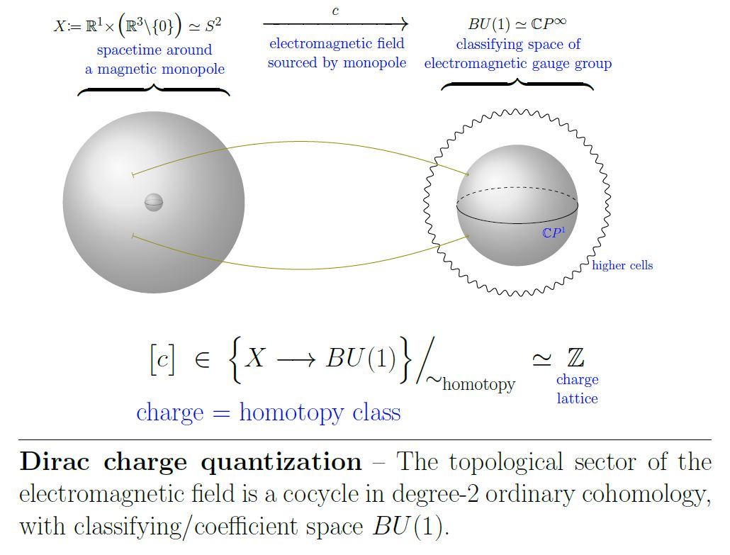
Dirac’s original argument

under construction

Dirac originally presented the following reasoning, which captures the main point of the above considerations.

He considered $X$ to be $\mathbb{R}^3$ without the origin,

$$X \coloneqq \mathbb{R}^3 \backslash \{0\} \,,$$

which is a manifold of the topology of (weakly homotopy equivalent to) the 2-sphere $S^2$.

He imagined a situation with a magnetic charge supported on the point located at the origin and removed that point in order to keep the field strength $F$ to be a closed 2-form on all of $X$.

(Indeed, if one does not remove the support of magnetic charge, the argument becomes much more sophisticated and involves higher differential cocycles given by bundle gerbes. This was not understood before Dan Freed’s Dirac charge quantization and generalized differential cohomology.)

Then he considered a single coordinate patch

$$U \coloneqq \mathbb{R}^3 \backslash \{x^1 \geq 0\} \subset X$$

given by $X$ minus the right half of the first coordinate axis.

Traditionally physicist try to give that half-line a physical interpretation by imagining that it is the body of an idealized infinitely-thin and to one side infinitely-long solenoid. Indeed, such a solenoid would have a magnetic monopole charge on each of its ends, so if the one end is imagined to have disappeared to infinity, then the other one is the magnetic charge that Dirac imagines to sit at the origin of our setup.

In this context the half-line $\{x^1 \geq 0\}$ is called a Dirac string. While there is the possibility to sensibly discuss the idea that this Dirac string actually models a physical entity like an idealized solenoid, its main purpose historically is to confuse physics students and keep them from understanding the theory of fiber bundles (see at fiber bundles in physics). Therefore here we shall refrain from talking about Dirac strings and consider $U \coloneqq \mathbb{R}^3 \backslash \{x^1 \geq 0\} \subset X$ as exactly what it is, by itself: an open subset that is part of a cover of $X$. Unfortunately, of course, Dirac didn’t mention the other open subsets in that cover (at least one more is needed for a decent discussion), so that the Dirac string keeps haunting physicists.

…running out of time…just quickly now…

…Dirac effectively considered the overlap cocycle condition $A_j - A_i = something$, found that by the requirement that $A$ has well defined holonomy it follows that there must be $g_{ij}$ a function with values in $U(1)$ such that $A_j - A_i = d log g_{ij}$, then did away with the $j$-patch (considering a kind of limit as we encircle the half axis) and concluded that $A$ must be the log-differential of a $U(1)$-valued function, whose winding number around the half-axis he identified with the magnetic charge, which in terms of bundles one identifies with the Chern-class of the bundle in question …

…have to run…

In modern terms:

The clutching construction gives $U(1)$-principal bundle ob $S^2$ by covering with two hemispheres $U_0$ and $U_1$ and picking a transition function $g \colon S^1 \to U(1)$ on the overlap $U_0 \cap U_1 \simeq S^1\times (0,\epsilon)$. The integral winding number of $g$ represents the first Chern class of the line bundle.

By the standard formula for existence of principal connections on given principal bundles, given a choice of partition of unity $\{\rho_i\}$ then the connection on $U_0$ is given by

$$A_0 = \rho_1 \mathbf{d} log g$$

If we think (as we may) of $U_0 = S^2 - \{\ast\}$ as covering most of the 2-sphere except one point and of $U_1$ the $\epsilon$-open neighbourhood of that point, then this $A_0$ vanishes on most of the sphere and close to the point taken out (“the Dirac string”) it becomes non-vanishing and equal to $g^{-1}\mathbf{d}g$.

Electric-magnetic charge quantization

Suppose we had a circle bundle with connection on a bundle representing an electromagnetic field with net magnetic charge $Q$ given by some magnetic current $j_{mag}$

$$d F = j_{mag}$$

that is supported in some compact spatial region $U \times \mathbb{R} \subset X$ with boundary sphere $\partial U \simeq S^2$.

$$q = \int_U j_{mag} = \int_U dF =\int_{\partial U} F = \int_{S^2} F$$

by the Stokes theorem. It follows from the fact that $F$ is the curvature 2-form on a circle bundle that $q$ is integral: it is given by the first Chern class of the bundle.

(…)

For $\gamma : S^1 \to X$ a closed but contractible trajectory of an electrically charged particle, the action functional is

$$\exp(i e \int_{S^1} \gamma^* A ) = \exp(i e \int_{D^2} \gamma^* F)$$

by the Stokes theorem, for some 2-disk cobounding the circle. If now $\gamma$ approaches a constant path and the 2-disk is taken to wrap the 2-cycle $\partial U$, then this becomes

$$1 = \exp(i e \int_{S^2} F) = \exp(i e q) \,.$$

Which implies that with the magnetic charge being quantized, also the electric charge is.

(…)

Related concepts

• fiber bundles in physics

• Dirac charge quantization

• dipole moment

• Hodge-Maxwell theorem

• quantum electrodynamics, Lamb shift

• Yang-Mills field

• Born-Infeld theory

• B-field, C-field

• ordinary differential cohomology, circle n-bundle with connection

• geometric origin of inhomogeneous media

References

Maxwell's equations originate in

• James Clerk Maxwell, A Dynamical Theory of the Electromagnetic Field, Philosophical Transactions of the Royal Society of London 155, 459–512 (1865).

Dirac's charge quantization argument appeared in

• P.A.M. Dirac, Quantized Singularities in the Electromagnetic Field, Proceedings of the Royal Society, A133 (1931) pp 60–72.

Review is for instance in

• Theodore Frankel, section 5.5 of The Geometry of Physics - An Introduction

Discussions of the basic geometry behind Maxwell equations can be found in

• Hong-Mo Chan, Sheung Tsun Tsou, Some elementary gauge theory concepts, gBooks
• Gregory L. Naber, Topology, geometry, and gauge fields: interactions
• Differential Forms in Electromagnetic Theory

For undergraduate lectures including experimental material see

• Walter Lewin, Electricity and magnetism, 2002, MIT opencourseware

The Lorentz-invariants of the electromagnetic field:

• C. A. Escobar, L. F. Urrutia, The invariants of the electromagnetic field, Journal of Mathematical Physics 55, 032902 (2014) (arXiv:1309.4185)