nLab geometry of physics
This page is growing incrementally as a series of lecture series proceeds.
Context
Physics
physics, mathematical physics, philosophy of physics
Surveys, textbooks and lecture notes
theory (physics), model (physics)
experiment, measurement, computable physics
-
-
-
Axiomatizations
-
Tools
-
Structural phenomena
-
Types of quantum field thories
-
Differential geometry
synthetic differential geometry
Introductions
from point-set topology to differentiable manifolds
geometry of physics: coordinate systems, smooth spaces, manifolds, smooth homotopy types, supergeometry
Differentials
Tangency
The magic algebraic facts
Theorems
Axiomatics
Models
differential equations, variational calculus
Chern-Weil theory, ∞-Chern-Weil theory
Cartan geometry (super, higher)
A set of lecture notes on differential geometry and theoretical fundamental physics, combining an introduction to traditional notions with an exposition of their formulation and refinement by higher geometry and extended prequantum field theory. With an eye towards Hilbert's sixth problem approached via cohesion.
Divided into two parts:
The geometry of fundamental physics is higher differential supergeometry.
| physics | mathematics |
|---|---|
| gauge principle | higher geometry (geometric homotopy theory) |
| Pauli exclusion principle | supergeometry |
Here:
-
Supergeometry is geometry whose spaces may have algebras of functions that are -graded-commutative algebras. This is the mathematical reflection of the Pauli exclusion principle, which says that a fermionic wave function on a phase space of a physical system with fermions has to have vanishing square. By linearity this implies that
and hence that fermionic wave functions anti-commute, and hence are the odd-graded elements in a commutative superalgebra (a slightly noncommutative algebra!)
Ever since the existence of fermionic particles was experimentally established, around the time of the Stern-Gerlach experiment in the 1920s, it is thus an experimental fact that fundamental physics is described by supergeometry. (This is not necessarily super-symmetric, though of course there is a close relation.)
-
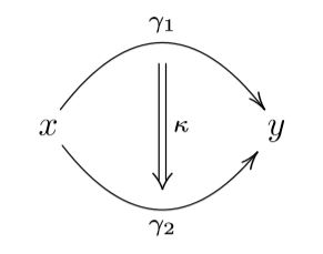
Higher structures is short for higher homotopy theoretic structures and reflects the gauge principle of physics: This says that, generally, it does not make invariant sense to ask if any two things , (e.g. field histories) are equal, instead one must ask for a gauge transformation between them, mathematically a homotopy:
This principle applies also to gauge transformations themselves, and thus leads to gauge-of-gauge transformations
and so on to ever higher gauge transformations:
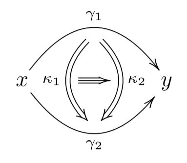
mathematically reflected by higher homotopies in higher homotopy types.
Ever since the existence of gauge fields was understood in the 1920s, it is thus an experimental fact that fundamental physics is described by higher geometry.
A striking consequence is that, both in higher geometry as well as in supergeometry and therefore in the geometry of fundamental physics, spaces generally are not sets of points, as in the traditional definition of topological spaces or differentiable manifolds.
What, then, is the geometry of fundamental physics?
The right framework to answer questions like this has been urged by Alexander Grothendieck already in Grothendieck 73 (see Lawvere 03) and has been much expanded on by William Lawvere (e.g. Lawvere 97, Lawvere 91) and has an evident lift to higher geometry (Lurie 09, S. 13), but has remained somewhat of a “public secret”:
The answer is known, alternatively, as (higher) functorial geometry (Grothendieck) or synthetic differential geometry in gros toposes (Lawvere), or variants thereof.
In this lecture series we try to give a self-contained introduction to higher differential supergeometry this way, following Schreiber 13. We begin at the beginning, with introducing relevant basics of category theory and topos theory and will provide brief indication of real-world applications to perturbative quantum field theory and fundamental super p-branes.
The higher differential geometry which we lay out subsumes various special cases that are discussed separately in the literature:
Notably diffeological spaces find home and company here: We explain how these are equivalently the concrete objects among the the bosonic smooth h-sets:
and we discuss how, even if one is initially interested only in ordinary smooth manifolds or only in diffeological spaces, it is useful to work with more general super differential homotopy types.

graphics taken from Higher Prequantum Geometry
Table
of chapters
Preliminaries
Part I) Geometry
Transition to part II
Part II) Physics
Contents
- About this text
- Categories and Toposes
- Smooth set
- Smooth homotopy types
- Stable homotopy types
- Groups
- Principal bundles
- Manifolds and Orbifolds
- -Structure and Cartan geometry
- Representations and Associated bundles
- Modules
- Flat connections
- de Rham Coefficients
- Principal connections
- Integration
- Super-geometry
- Prequantum geometry
- WZW terms
- BPS charges
- Perturbative quantum field theory
- Physics in Higher Geometry: Motivation and Survey
- Hamilton-Jacobi-Lagrange mechanics via prequantized Lagrangian correspondences
- Hamilton-de Donder-Weyl field theory via Higher correspondences
- Local (topological) prequantum field theory
- Prequantum Gauge theory and Gravity
- Quantum mechanics
- Geometric quantization
- Model Layer
- 1-Geometric quantization
- Geometric quantization with KU-coefficients
- Quantum 3d Chern-Simons theory for compact simple gauge group
- Higher geometric quantization
- Semantics Layer
- Syntactic Layer
- Application to open questions in physics
- Related expositions
- References
- General
About this text
This page is going to contain an introduction to aspects of differential geometry and their application in fundamental physics: the gauge theory appearing in the standard model of particle physics and the Riemannian geometry appearing in the standard model of cosmology, as well as the symplectic geometry appearing in the quantization of both.
Scope and perspective
The intended topic scope and readership of the first layer of this page – the Model Layer – is much like that of the book (Frankel), only that here we make use of a more modern and more transparent conceptual toolbox. We also discuss in two other layers, the Semantic Layer and the Syntactic Layer deeper mechanisms at work in the background.
Notably, where traditional expositions of differential geometry proceed by generalizing the geometry of abstract coordinate systems to smooth manifolds, here we instead begin by generalizing, in Smooth sets – Model Layer, coordinate systems right away to smooth sets, which happens to be both more expressive as well as actually much easier. In parallel (and to be read independently or not at all) we discuss in Smooth sets – Semantic Layer how this means that we are working in the sheaf topos over abstract coordinate systems. Smooth manifolds are then introduced later as an intermediate notion, together with that of diffeological spaces. (Many of the constructions in differential geometry applied in physics do not actually need the notion of a smooth manifold, and, more importantly, for many notions in modern theoretical physics smooth manifolds are not actually sufficiently general.)
In fact we introduce smooth manifolds only after we introduce smooth groupoids (below in Smooth homotopy type - Model Layer - Smooth groupoids), which are differential geometric structures that are still simpler than smooth manifolds, and of course even more expressive than smooth sets. Moreover, smooth groupoids are at the very heart of the geometry of physics: modern fundamental physics is all based on the “gauge principle” and in Model Layer – Gauge transformations in electromagnetism we explain how, mathematically, this is essentially nothing but the theory of smooth groupoids. As further background information we discuss in Smooth homotopy types - Semantic Layer how this means that we are working in a higher topos over abstract coordinate systems, and in Smooth homotopy type - Syntactic Layer how this means that we are reasoning about physics using the natural deduction rules of homotopy type theory.
From this setup then naturally flow all the many structures and phenomena seen in the geometry of physics:
Layers of exposition
We discuss each topic below in three stages, in three layers.
- The first layer, called the Model Layer, deals with concrete explicit constructions as familiar from traditional textbooks on differential geometry and physics. This layer is supposed to be readable and useful all in itself and the reader who feels that this is all he or she wants to see can stick to this and ignore the other layers. In particular, while the Model Layer does invoke the basic notion of a category and of a functor – which are as simple as the notions of group or algebra –, it does not use any actual category theory.
- The second layer, called the Semantic Layer, makes explicit the (higher) category theory and (higher) topos theory at work in the background. This puts the concrete constructions of the Model Layer into a more general context and helps to see certain organizational patterns that underlie the seemingly different phenomena. It provides some powerful theorems which the Model Layer is secretly benefitting from. For instance this layer gives a systematic rule for generalizing everything at the beginning Model Layers from ordinary differential geometry to what is called supergeometry, which is the context in which fermionic particles are formalized: the matter constituents of the observable universe.
- The third layer, called the Syntactic Layer, makes explicit the expression of these phenomena in the formal internal language of the topos of smooth sets – which is dependent type theory – and of the higher topos of smooth higher groupoids – which is homotopy type theory. This makes more transparent various constructions in (higher) topos theory used in Semantic Layer, and in fact it provides a natural construction principle for objects in a (higher) topos that model some intended meaning – which is precisely what mathematical physics is all about. This is meant for readers who enjoy seeing fundamental physics naturally rooted in genuinely fundamental mathematics, in natural deduction from practical foundations, as it were. Everybody else should ignore this.
The three layers
-
Model Layer – concrete particular: models
-
Semantic Layer – concrete general: categorical semantics in higher topos theory
-
Syntactic Layer – abstract general: syntax in homotopy-type theory
This topos-theoretic perspective on fundamental physics which is discussed here is mostly original in the identifications it makes (Schreiber), but it draws insights and inspiration from (and maybe realizes) a vision already expressed since the 1960s by William Lawvere, one of the central figures in the development of topos theory and categorical logic. Lawvere links the very inception of topos theory to the motivation to axiomatize physics:
My own motivation for developing topos theory came from my earlier study of physics. The foundation of the continuum physics of general materials, involves powerful and clear physical ideas which unfortunately have been submerged under a mathematical apparatus including not only Cauchy sequences and countably additive measures, but also ad hoc choices of charts for manifolds and of inverse limits of Sobolev Hilbert spaces, to get at the simple nuclear spaces of intensively and extensively variable quantities. But, as Fichera lamented, all this apparatus may well be helpful in the solution of certain problems, but can the problems themselves and the needed axioms be stated in a direct and clear manner? And might this not lead to a simpler, equally rigorous account? (Lawvere, 2000)
More historical pointers along these lines and further related material can also be found at higher category theory and physics.
To give a survey of how the exposition below proceeds in the fashion of these three layers, the following section The full story in a few formal words provides what may be read as commented index to the central themes of the following text. Whereas the exposition below is organized to start each topic with the discussion of its concrete models in a Model layer, then pass to a general abstract semantics in a Semantic Layer and then finally to the abstract formal syntax in a Syntactic Layer, these tables indicates how this passage to abstract syntax usefully reflects back onto the concrete theory:
The leftmost columns of the following tables formulate concepts in terms of ordinary language. The second columns translate that ordinary language fairly directly to the formal language of (homotopy) type theory. The third columns then interprets these formal syntactical expressions as universal constructions in a (higher, cohesive) topos by the rules of categorical semantics. Finally, the fourth columns indicate what this universal construction amounts to when concretely realized in the model given by smooth sets and smooth ∞-groupoids. Finally the rightmost columns point to the chapters in the text below that deal with the given construction.
These tables show that fairly evident and naïve sounding statements in ordinary language turn under this translation into what is generally regarded as fairly sophisticated constructions. In fact some of these constructions have only been found by translating along the categorical semantics dictionary this way. So the following tables also serves to show how the general abstract discussion here is a means to facilitate reasoning about seemingly complicated concepts underlying fundamental physics:
The full story in a few formal words
We give an overview in the spirit of Synthetic Quantum Field Theory.
The fundamental physics of the observed world is governed by what is called quantum theory. (This is explicitly so for the standard model of particle physics and induced from this all fundamental physics ever tested in laboratories; but by all that is known also the remaining ingredient of gravity is fundamentally a quantum theory, see at quantum gravity for comments).
Two major axiomatizations of quantum theory are known, namely
-
FQFT where one axiomatizes the assignment of spaces of states to pieces of worldvolume (the “Schrödinger picture” of quantum theory)
fragments of which involve:
-
finite quantum mechanics in terms of dagger-compact categories
-
FRS-construction of 2d CFT from this via holography
-
-
AQFT where one axiomatizes the assignment of algebras of observables to pieces of worldvolume (the “Heisenberg picture” of quantum theory)
fragments of which involve:
(For an attempt at a survey of the state of the art as of 2011 see the collection (Sati-Schreiber)).
But all fundamental quantum field theories observed in (or conjectured to underlie) nature arise by a process called quantization from structures in differential geometry (or are induced via a mechanism called the holographic principle from such that do).
This differential geometric data involves
-
smoothfunctionals – called action functionals
-
on smooth "spaces" – called moduli stacks
-
of differential geometric structures such as fiber bundles and connections – called gauge force fields
-
as well as sections of associated bundles – called matter fields.
Similar differential geometric structures are involved in the geometric quantization of such an action functional to an actual quantum field theory.
Hence there is a sequence:
| differential geometry | geometric quantization | quantum field theory |
|---|
We discuss a formalization of central aspects of this entire sequence. Our development proceeds – as befits a theory of physics and hence of nature – via natural deduction from practical foundations.
Fundamentally, a language for physics is to be a language about existence; a language in which we can express judgements of the form:
There is a thing of type .
For instance:
There is a gauge field in the standard model of gauge fields on spacetime .
(Here the square bracket expression for a moduli stack of gauge fields will be incrementally explained in the following.)
To be predictive, a language for physics is moreover to be a language in which we can make natural deductions to deduce further such judgements from given ones. For instance:
Given a gauge field as above, there is an underlying instanton sector, , in the collection of instanton configurations in the standard model.
Quantum superpositions of such Yang-Mills instantons are the very substrate out of which the vacuum of the observed world is build: the instanton liquid in quantum chromodynamics. (For more see at Yang-Mills theory below.) We consider here a language to reason about such phenomena formally.
The formal language for such natural deduction of judgements about there being terms of some type is called type theory.
Expressions in (dependent) type theory:
(read columns 1+2 first, then 3+4)
| ordinary language | syntax | semantics | model | chapter |
|---|---|---|---|---|
| general abstract | general concrete | concrete particular | ||
| There is… | (We speak in the context of a (higher) topos , a place where things may be. (For the time being a (higher) locally cartesian closed category is sufficient.)) | (A topos for synthetic differential geometry, such as ShSmthMfd. Eventually a higher such topos: Smooth∞Grpd or SynthDiff∞Grpd or SmoothSuper∞Grpd or …) | Smooth sets and Smooth homotopy types | |
| There is a thing of type . | An element of an object of . | A point in a smooth moduli stack . | Judgements about types and terms | |
| There is a type of things . | An element of the small-object classifier of . | A point in the moduli stack of all small moduli stacks. | Judgements about types and terms | |
| Given a thing of type there is a thing of type | An element of a morphism in the slice topos . | An -family in a moduli stack bundle over . | Slice categories and Slice toposes and Slice ∞-Toposes | |
| There is the collection of all things for all . | The dependent sum/left adjoint to the product: | The total space of a bundle. | Natural deduction rules for dependent sum types | |
| There is a thing in the collection of all things for all . | An element of the total space object. | A point in the moduli stack over . | ||
| There is an assignment of an to each . | . | An element in the internal object of sections | A point in the smooth relative mapping space of smooth sections. | Natural deduction rules for dependent product types |
| There is the collection of assignments of an to each . | internal space of sections | A smooth relative mapping space of smooth sections. | ||
| In particular, there is the collection of such assignments when does not depend on , the collection of functions from to . | The internal hom object . | A smooth mapping space. | Smooth mapping spaces and smooth moduli spaces | |
| There is a proof that it is true that there is of type . | An element of the (-1)-truncation of the object . | A point in the smooth sets of equivalence classes of points in . | Subobjects | |
| There is a proof that it is true that there is an for some . |
In order to describe a structured reality, our language needs to be able to speak about comparison of things.
Fundamental physics rests on the gauge principle: it is meaningless to say that two things – such as two gauge fields as above – are equal; instead they are gauge equivalent if there is a gauge transformation between them.
So our language needs to express judgements of the form:
There is a gauge equivalence between gauge fields and .
And the language needs to be able to make natural deductions from such judgements to arrive at:
Given an equivalence there is an equivalence between the underlying instanton sectors.
The formal language based of the dependent type theory which we have so far that contains these statements is type theory with propositional equality. In this language we have judgements such as the following.
Expressions in dependent type theory with propositional equality:
| ordinary language | syntax | semantics | model | chapter |
|---|---|---|---|---|
| general abstract | general concrete | concrete particular | ||
| Given , there is the collection of equivalences between and equivalent. | . | The mapping cocone object | The moduli stack of gauge transformations between and . | Identity types |
| There is an equivalence between and . | An element of the mapping cocone object. | A gauge transformation between and . | ||
| Given , there is the collection of proofs that it is true that and are equivalent. | . | The (-1)-truncation fo the mapping cocone. | The smooth set of equivalence classes of gauge transformations from to . |
But the gauge principle reaches deeper: gauge transformations themselves are subject to the gauge principle.
In general it is meaningless to ask if two gauge transformations are equal, but we may ask if there is a higher gauge transformation that transforms one gauge transformation into the other. In the physics literature such gauge-of-gauge transformations are best known in their incarnation as ghost-of-ghost fields in what is called the BRST complex of the given gauge theory.
Careful analysis for instance of the Dirac charge quantization of magnetic charge shows that already quite mundane physical phenomena exhibit such higher gauge transformations. But more famously they are known to arise in various guises in string theory, which is a hypothetical refinement of the standard model of particle physics and gravity.
In either case, our formal language should not allow the deduction that gauge equivalences are themselves either equal or not, but only allow judgements of the following form:
There is a gauge-of-gauge equivalence between two given gauge equivalences between two given gauge fields .
The flavor of type theory with propositional equality for which this is the case is called intensional type theory.
Since therefore a type in intensional type theory may contain homotopies between its terms of arbitrary order, we call it a homotopy type.
The homotopy-type nature of the type of gauge connections is most familiar in the physics literature in its infinitesimal approximation, which is the (off-shell) BRST complex of the gauge theory: the -fold ghost-of-ghost fields in the BRST complex correspond to the -fold homotopies in .
In particular, in intensional type theory we find the gauge group of a homotopy type, as indicated in the following table.
Expressions in intensional type theory:
| ordinary language | syntax | semantics | model | chapter |
|---|---|---|---|---|
| general abstract | general concrete | concrete particular | ||
| Given a type , there is (the underlying space) of a group of ways that is equivalent to itself. | A loop space object | A smooth ∞-group. | n-groups | |
| Given a function between collections of things and , and given a thing , there is its preimage-up-to-equivalence. | A homotopy pullback | The homotopy fiber of a homomorphism of smooth moduli stacks. |
Suppose then that we have such a map between collections of gauge fields
on two possibly different spacetimes with two possibly different gauge groups.
(For instance we might be looking at Montonen-Olive duality/_S-duality_ or Seiberg duality of super Yang-Mills theory.)
Then we should call an equivalence - in the physics literature often: a duality – if, while not necessarily being a “bijection”, it is such that the preimage of a gauge field consists of gauge fields that are all gauge equivalent to each other, with the gauge equivalences exhibiting this equivalence themselves all being gauge equivalent to each other, etc.
If this is the case one says that all homotopy fibers – all gauge pre-images – of are contractible – are gauge equivalent to a single gauge field – and that is a weak homotopy equivalence.
For consistency we should demand that the notion of equivalence is such that the space of direct equivalences is itself equivalent to the space of such weak homotopy equivalences (“dualities”) .
This requirement is called the univalence axiom. The intensional type theory-language considered so far equipped with this axiom is called homotopy type theory.
We indicate now some central judgements that are expressible in homotopy type theory. This involves fundamental judgements in group theory and in representation theory, two of the pillars of modern quantum theory/quantum field theory.
Structures expressible in homotopy type theory:
| ordinary language | syntax | semantics | model | chapter |
|---|---|---|---|---|
| general abstract | general concrete | concrete particular | ||
| Given a type , there is a group of ways that is equivalent to itself. | A loop space object | A smooth automorphism ∞-group. | n-groups | |
| Given a type , there is the delooping of , which is the collection of things equipped with equivalences to . | The looping and delooping relation | The smooth moduli stack of smooth -principal ∞-bundles. | Principal n-bundles | |
| Given a thing in , there is a thing . | A homotopy fiber sequence with homotopy fiber over . | An ∞-action/∞-representation of on some , together with its universal -associated -fiber ∞-bundle over the moduli stack for -principal ∞-bundles. | Higher actions | |
| Given a function classifying a -principal bundle and given a point in the delooping, there is the -principal bundle itself, being the collection of identifications of the fiber with | The principal ∞-bundle given as the homotopy pullback of the universal principal ∞-bundle. | Principal ∞-bundles | ||
| There is a -equivariant map from the principal bundle to the representation space. | An element of in the slice topos | A section of the -associated -fiber ∞-bundle. |
In gauge theory physics, a representation of the gauge group encodes the particle-content of the model (in theoretical physics): a section of the -associated bundle to the gauge bundle is a matter field in the model.
Therefore all the ingredients so far encode the kinematics of gauge theory, its setup before an actual dynamics is specified.
Dynamics in physics says how things move, hence how they trace out trajectories in a given spacetime or more generally in some phase space.
Our language for reasoning about physics should be able to express this. For a homotopy type that models spacetime (the collection of all points of spacetime) there should be a homotopy type whose homotopies and higher homotopies are the smooth trajectories, the smooth paths and higher paths in .
In order to analyse the notion of smoothness here – we will say: the way that points hold together by cohesion – there should also be
-
an expression for the discrete collection of points underlying – detaching all points;
-
an expression which dissolves the cohesion and produces the codiscrete smooth structure on .
There are some natural simple axioms on these constructions. For instance every smooth path in a discrete space should be constant: .
With such natural axioms understood, these three constructions constitute an adjoint triple of modalities in our language. In particular and are a monad and comonad on the type system, in the sense of computer science and is even an internal monad.
Equipping the above homotopy type theory with these modalities turns it into what we call cohesive homotopy type theory.
Structures expressible in cohesive homotopy type theory:
| ordinary language | syntax | semantics | model | chapter |
|---|---|---|---|---|
| general abstract | general concrete | concrete particular | ||
| Given a cohesive homotopy type , there is the dissolved homotopy type in which all separate points are collected to one cohesive blob. | The codiscrete object-monad on a (higher) local topos. | The codiscrete smooth structure on the points of . | Locality of the topos of smooth spaces | |
| Given a cohesive homotopy type, there is the map that dissolves the cohesion of the points. | The unit of the codiscrete object monad. | The function that sends smooth families in a smooth moduli stack to families of points. | ||
| Given there is the collection of points in and smooth trajectories between points in . | The construction of the fundamental ∞-groupoid in a locally ∞-connected (∞,1)-topos. | The smooth path ∞-groupoid of . | The local ∞-connectedness of the (∞,1)-topos of smooth ∞-groupoids | |
| Given , there is a canonical map to . | . | The unit of the -monad on a locally ∞-connected (∞,1)-topos. | The inclusion of into its smooth path ∞-groupoid as the constant paths. | |
| Given , there is the result of detaching the points in . | The operation of the discrete object comonad on a (higher) local topos. | The moduli stack for flat ∞-connections. | ||
| Given , there is a map from flat -connections to the underlying -bundles | The counit of the discrete object-comonad on a (higher) local topos. | The function that sends a flat ∞-connection to its underlying principal ∞-bundle. | Flat connections |
Adding the modalities to the above language of homotopy type theory yields a language that we call cohesive homotopy type theory (following a term introduced by Lawvere).
Fundamental judgements in cohesive homotopy type theory include those indicated in the following table, which capture central concepts of gauge theory and its (higher) geometric quantization.
Structures expressible in cohesive homotopy type theory:
Gauge fields, matter fields, and smooth action functionals on their moduli stacks…
| ordinary language | syntax | semantics | model | chapter |
|---|---|---|---|---|
| general abstract | general concrete | concrete particular | ||
| A flat connection on is a rule for sending paths to group elements, respecting composition. | . | The higher parallel transport of a flat connection : a (higher) gauge field with vanishing field strength. | Flat connections | |
| A closed differential form is a flat connection and a trivialization of the underlying bundle. | The coefficients for de Rham hypercohomology – flat ∞-Lie algebra valued differential forms. | de Rham coefficients | ||
| A general connection is the equivalence between the curvature of a bundle and a closed differential form . | The coefficients for smooth differential cohomology: abelian (higher) gauge fields. | Circle principal n-connections | ||
| There is a cohesive function from -gauge fields to higher -gauge fields. | A differential universal characteristic class. | An extended action functional/prequantum n-bundle for extended higher Chern-Simons-type gauge theory. |
… and their ∞-geometric prequantization (see there for a more comprehensive dictionary):
| ordinary language | syntax | semantics | model | chapter |
|---|---|---|---|---|
| general abstract | general concrete | concrete particular | ||
| There is a -equivariant map from the prequantum bundle to the representation space. | A prequantum state. | Geometric quantization | ||
| There is a differentially -equivariant equivalence from the prequantum bundle to itself. | A prequantum operator: an element of the quantomorphism group/Heisenberg group of the quantum system. | Geometric quantization |
Finally, in order to be able to concretely speak about not just about any gauge field, but the concrete particular gauge fields in the observable universe, our language should be able to express the existence of the continuum real line.
| ordinary language | syntax | semantics | model | chapter |
|---|---|---|---|---|
| general abstract | general concrete | concrete particular | ||
| There is the continuum line. | line object | real line | The continuum real worldline |
This then induces the existence of the circle group . The electromagnetic field is a gauge field for gauge group . Therefore in the language of cohesive homotopy type theory we can say
Let there be light.
| ordinary language | syntax | semantics | model | chapter |
|---|---|---|---|---|
| general abstract | general concrete | concrete particular | ||
| There is the collection of higher -principal connections. | The coefficients for ordinary differential cohomology (with coefficients in an Eilenberg-MacLane object.) | The smooth higher moduli stack of smooth circle n-bundles with connection. | Circle-principal n-connections. | |
| There is light. | A cocycle in ordinary differential cohomology in degree-2. | A configuration of the electromagnetic field on spacetime . | Circle principal connection |
There are of many more constructions in fundamental (quantum) physics that are naturally expressible in cohesive homotopy type theory, but the above should already give an idea and highlight the cornerstones of the following discussion.
We now end this introduction and overview and turn to the in-depth account of geometry of physics.
Contents
I) Geometry
We begin by laying the foundations of differential geometry. Doing this in the natural abstract way seamlessly leads over to the foundations of higher differential geometry (see also motivation for higher differential geometry). Once this is set up, we discuss the fundamental constructions: groups, actions/representations, fiber bundles, connections, Chern-Weil theory.
Categories and Toposes
This chapter is as geometry of physics – Categories and Toposes
Smooth set
This chapter is at geometry of physics – smooth sets.
Smooth homotopy types
This chapter is at geometry of physics – smooth homotopy types.
Stable homotopy types
This chapter is at geometry of physics – stable homotopy types.
Groups
This chapter is at geometry of physics – groups.
Principal bundles
This chapter is at geometry of physics – principal bundles.
Manifolds and Orbifolds
this chapter is at geometry of physics – manifolds and orbifolds
-Structure and Cartan geometry
this chapter is at geometry of physics – G-structure and Cartan geometry
Representations and Associated bundles
this chapter is at geometry of physics – representations and associated bundles
Modules
this chapter is at geometry of physics - modules
Flat connections
this chapter is at geometry of physics – flat connections
de Rham Coefficients
see geometry of physics – de Rham coefficients
Principal connections
this chapter is at geometry of physics – principal connections
Integration
this chapter is at geometry of physics – integration
Super-geometry
this chapter is at geometry of physics – supergeometry and superphysics
Prequantum geometry
this chapter is at geometry of physics – prequantum geometry
WZW terms
this chapter is at geometry of physics – WZW terms
BPS charges
this chapter is at geometry of physics – BPS charges
Contents
II) Physics
Perturbative quantum field theory
This section is at geometry of physics – perturbative quantum field theory.
Physics in Higher Geometry: Motivation and Survey
Before we discuss technical details starting in the next chapter here we survey general ideas of theories in fundamental physics and motivate how these are naturally formulated in terms of the higher geometry that we developed in the first part.
This chapter is at geometry of physics – physics in higher geometry.
Hamilton-Jacobi-Lagrange mechanics via prequantized Lagrangian correspondences
This chapter is at prequantized Lagrangian correspondence.
Hamilton-de Donder-Weyl field theory via Higher correspondences
This chapter is at Local field theory via Higher correspondences.
Local (topological) prequantum field theory
This chapter is at geometry of physics – local prequantum field theory.
Prequantum Gauge theory and Gravity
this chapter is at geometry of physics – prequantum gauge theory and gravity
Quantum mechanics
This section is at geometry of physics – quantum mechanics
Geometric quantization
Model Layer
1-Geometric quantization
Geometric quantization with KU-coefficients
this is at geometric quantization with KU-coefficients
Quantum 3d Chern-Simons theory for compact simple gauge group
Higher geometric quantization
Semantics Layer
Syntactic Layer
(…)
Application to open questions in physics
What is it that higher geometry, higher gauge theory, extended/local field theory and generally higher category theory in physics contribute to open research questions in theoretical physics?
Often when this question is asked the most glaring open question of contemporary theoretical physics is forgotten:
What IS local quantum field theory?
While something going by this name is clearly in use, it is just as clear that the full answer to this question is only being discovered these days, with formalizations such as the cobordism theorem and constructions such as factorization algebras in BV-quantization – both of which are crucially constructions in higher geometry/higher category theory.
Despite the huge success of quantum field theory, it it worthwhile to remember that all the fundamental open questions in present day fundamental physics quite likely require a deeper understanding of what quantum field theory actually is, notably non-perturbatively:
-
Why is there confinement/chiral symmetry breaking in non-perturbative QCD/Yang-Mills theory? (The “mass gap problem”.)
-
What is beyond-the-standard-model physics?
-
What is quantum gravity?
-
What is non-perturbative string theory?
For instance the standard model of cosmology says that the bulk of all energy and matter in the observable universe is entirely unknown to us (dark matter, “dark energy”), while at the same time the theoretical prediction what the cosmological constant vacuum energy should be is entirely off. How glaring an open question about the nature of quantum field theory this actually is is often forgotten due to the success of effective field theory-type of reasoning that allows to neatly wrap up all this unknown energy into a single term in some effective equation. Phenomenologically this may be regarded as a success, but for fundamental theoretical physics it is a glaring open question.
And while there is work going in this direction, it may be worthwhile to recall how relatively primitive the available theoretical tools often still are. For instance it seems clear that “canonical non-covariant quantization” can hardly be an approrpiate tool to approach anything in the direction of quantum gravity. Even so fundamental a notion as that of covariant phase space necessary to make progress here is not widely known in the theoretical physics community. Attempts to refine quantization to a “covariant” and “local” formalism via multisymplectic geometry have mainly got stuck, since local observables just do not form a sensible structure in ordinary Lie theory. This is resolved only in infinity-Lie theory and higher differential geometry, as discussed above (hgp 13, lo 13).
If one assumes that string theory is part of the answer as to what underlies the standard model of particle physics and cosmology, then this situation becomes more drastic even. The fundamental fields of string theory are clearly objects in higher differential geometry, such as the B-field, the RR-field, the supergravity C-field etc. For instance the natural identification of the latter as a homotopy fiber product of moduli stacks in (FSS7dCS, FSSCField) is hardly conceivable when ignoring higher differential geometry. And this is a structure meant to be at the very heart of what makes up string theory. It is unlikely that the landscape of string theory vacua and hence the relation of string theory to phenomenology can really be understood if such basic higher-geometric phenomena of string theory are ignored (see Distler-Freed-Moore 09 on this point).
(…)
Related expositions
References
{}
General
A textbook with basic introductions to differential geometry and physics is
A discussion of aspects of quantum field theory with emphasis on the kind of modern tools that we are using here is in
- Frédéric Paugam, Towards the mathematics of quantum field theory (pdf)
The present discussion corresponds to section “1.2 Geometry of phyics” in
which gives a more comprehensive account.
Another set of lecture notes along the above lines with an emphasis on aspects in gravity and higher gauge theory motivated from string theory is in
- Urs Schreiber, twisted smooth cohomology in string theory, Lectures notes at Quantum Fields and twisted K-theory, ESI (2012)
An exposition and survey of matters related to Chern-Simons theory and higher geometric quantization is in
The syntactic perspective above is laid out further in
see also at motivic quantization the section General abstract type theoretic summary.
Mathematical quantum field theory
A textbook (really a collection of lecture notes) on quantum field theory and string theory that tries to present material in a conceptually clean way is
- Pierre Deligne, Pavel Etingof, Dan Freed, L. Jeffrey,
David Kazhdan, John Morgan, D.R. Morrison and Edward Witten, eds. Quantum Fields and Strings, A course for mathematicians, 2 vols. Amer. Math. Soc. Providence 1999. (web version)
A collection trying to summarize the state of the art of the formalization of QFT by FQFT and AQFT as of 2011 is
- Hisham Sati, Urs Schreiber, Mathematical Foundations of Quantum Field and Perturbative String Theory, Proceedings of Symposia in Pure Mathematics, volume 83 AMS (2011)
Topos theory in differential geometry and physics
One of the central figures of topos theory and categorical logic, William Lawvere, has motivated his interest in these subject always with intended application to the formalization of physics (of classical continuum mechanics in his case).
An influential text is
- William Lawvere, Toposes of laws of notion, Toposes of laws of motion , transcript of a talk in Montreal, Sept. 1997 (pdf)
which motivates synthetic differential geometry from differential equations appearing as equations of motion in physics. The early text
- William Lawvere, Some Thoughts on the Future of Category Theory in A. Carboni, M. Pedicchio, G. Rosolini, Category Theory , Proceedings of the International Conference held in Como, Lecture Notes in Mathematics 1488, Springer (1991)
already sketches the formulation of cohesive toposes and motivates their axioms with heuristics from geometry and physics.
A review by Lawvere is in
- William Lawvere, Comments on the Development of Topos Theory, Development of Mathematics 1950-2000, 715-734 (2000) Birkhäuser Basel
Modern accounts of physics in this spirit includes notably also the book (Paugam) listed above.
Higher category theory in physics
An early proposal that the action functional of -dimensional quantum field theory should refine to a structure involving (n-k)-vector spaces in codimension is in
The full formalization of this for extended topological field theory is due to
Related comments on the extended quantization of infinity-Dijkgraaf-Witten theory are in
- Daniel Freed, Michael Hopkins, Jacob Lurie, Constantin Teleman Topological Quantum Field Theories from Compact Lie Groups
For more pointers see at higher category theory and physics.
Local prequantum field theory
The idea of formulating local prequantum field theory by spans in a slice over a “space of phases” in higher geometry has been expressed in the unpublished note
A formulation of the idea for Dijkgraaf-Witten theory-type field theories is indicated in section 3 of
- Daniel Freed, Michael Hopkins, Jacob Lurie, Constantin Teleman, Topological Quantum Field Theories from Compact Lie Groups (2010)
based on the considerations in section 3.2 of
Based on the general formulation of the more general field theory with defects described in section 4.3 there, in
- Domenico Fiorenza, Alessandro Valentino, Boundary conditions in local TFTs (in preparation)
the structure of such domain walls/defects/branes are analyzed in the prequantum theory, hence with coefficients in an (∞,n)-category of spans.
The study of local prequantum ∞-Chern-Simons theory with its codimension-1 ∞-Wess-Zumino-Witten theory and codimension 2-Wilson line-theory in this fashion, in an ambient cohesive (∞,1)-topos is discussed in (lpqft)
Much of the content of this entry here are, or arose as, lecture notes for
- Urs Schreiber, Higher Chern-Simons theory Introduction, at the workshop Chern-Simons Theory: Geometry, Topology and Physics University of Pittsburgh (May 2013)
Higher geometric prequantum theory
- Domenico Fiorenza, Chris Rogers, Urs Schreiber, L-∞ algebras of local observables from higher prequantum bundles
Further details
Physical fields
For references on the tradtional formulation of physical fields by sections of field bundles as discussed above see there references there.
The formulation of physical fields as cocycles in twisted cohomology in an (∞,1)-topos as in the Definition-section above originates around
- Urs Schreiber, Background fields in twisted differential nonabelian cohomology, talk at Oberwolfach Workshop, June 2009 – Strings, Fields, Topology
Further articles since then are listed at
In particular the general notion of fields as twisted differential c-structures appears in
- Hisham Sati, Urs Schreiber, Jim Stasheff, Twisted Differential String and Fivebrane Structures (arXiv:0910.4001)
and the general theory of cohomology and twisted cohomology with local coefficient ∞-bundles as referred to in Relation to twisted cohomology above as well as the theory of associated ∞-bundles as in Sections of associated ∞-bundles is laid out in
- Thomas Nikolaus, Urs Schreiber, Danny Stevenson, Principal ∞-bundles – theory, presentations and applications (arXiv:1207.0248)
Some examples of fields in this sense are called “relative fields” in
- Daniel Freed, Constantin Teleman, Relative quantum field theory (arXiv:1212.1692)
Differential forms and parallel transport
The relation between differential 1-forms and smooth incremental path measures as used above is discussed in
- Urs Schreiber, Konrad Waldorf, Parallel transport and functors, J. Homotopy Relat. Struct. 4, 187-244 (arXiv:0705.0452)
For a commented list of related literature see here.
(…)
3d Chern-Simons theory and Wilson loops
- Chris Beasley, Localization for Wilson Loops in Chern-Simons Theory, in J. Andersen, H. Boden, A. Hahn, and B. Himpel (eds.) Chern-Simons Gauge Theory: 20 Years After, , AMS/IP Studies in Adv. Math., Vol. 50, AMS, Providence, RI, 2011. (arXiv:0911.2687)
Higher Chern-Simons theories
The discussion of the abelian 7d Chern-Simons theory involved in AdS7/CFT6 duality is due to (Witten 98). A discussion of the non-abelian quantum-corrected and extended refinement is in
Construction of differential cup-product theories is in
Last revised on June 11, 2022 at 10:28:46. See the history of this page for a list of all contributions to it.