nLab linear logic
Context
Foundations
The basis of it all
Set theory
- fundamentals of set theory
- material set theory
- presentations of set theory
- structuralism in set theory
- class-set theory
- constructive set theory
- algebraic set theory
Foundational axioms
-
basic constructions:
-
strong axioms
-
further
Removing axioms
Type theory
natural deduction metalanguage, practical foundations
type theory (dependent, intensional, observational type theory, homotopy type theory)
computational trinitarianism =
propositions as types +programs as proofs +relation type theory/category theory
Monoidal categories
With braiding
With duals for objects
-
category with duals (list of them)
-
dualizable object (what they have)
-
ribbon category, a.k.a. tortile category
With duals for morphisms
-
monoidal dagger-category?
With traces
Closed structure
Special sorts of products
Semisimplicity
Morphisms
Internal monoids
Examples
Theorems
In higher category theory
Contents
Idea
Linear logic is a substructural logic in which the contraction rule and the weakening rule are omitted, or at least have their applicability restricted.
Absence of weakening and contraction
Notice that contraction and weakening are the two structural inference rules which exhibit context extensions as admitting natural diagonal and projection maps, respectively, hence as admitting interpretation as cartesian products (cf. Jacobs 1994):
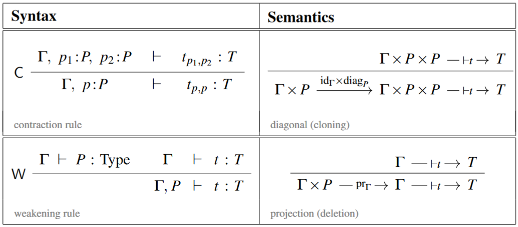
Therefore, when these inference rules are dropped then the resulting multiplicative conjunction of contexts may still have interpretation as a symmetric monoidal tensor product (such as known from the tensor product of vector spaces) but not necessarily as a cartesian monoidal product (such as known from the product of topological spaces).
Accordingly, if implication still follows the usual inference rule of function types but now with respect to a non-cartesian multiplicative conjunction
etc., then the function type may be interpreted as an internal hom in a non-cartesian closed monoidal category with symmetric monoidal tensor product — such as the category of finite-dimensional vector spaces, in which case the terms interpret as linear functions — whence the logical connective “” is also called linear implication.
Which exact flavour of monoidal category provides categorical semantics for linear logic depends on exactly which further inference rules are considered (see also at bunched logic): In the original definition of Girard (1987), linear logic is the internal logic of/has categorical semantics in star-autonomous categories (Seely 89, prop. 1.5). But more generally linear logic came to refer to the internal logic of any possibly-non-cartesian symmetric closed monoidal category (then usually called multiplicative intuitionistic linear logic – MILL) or even polycategory (Szabo 78 see the history section and see also de Paiva 89, Blute 91, Benton–Bierman–de Paiva–Hyland 92, Hyland–de Paiva 93, Bierman 95, Barber 97, Schalk 04, Melliès 09). Under this interpretation, proof nets (or the associated Kelly–Mac Lane graphs) of linear logic are similar to string diagrams for monoidal categories.
Indeed, these more general senses of linear logic still faithfully follow the original motivation for the term “linear” as connoting “resource availability” explained below, since the non-cartesianness of the tensor product means the absence of a diagonal map and hence the impossibility of functions to depend on more than a single (linear) copy of their variables.
In addition to these usual “denotational” categorical semantics, linear logic also has an “operational” categorical semantics, called the Geometry of Interaction, in traced monoidal categories.
Although linear logic is traditionally presented in terms of inference rules, it was apparently discovered by Girard while studying coherence spaces.
As a quantum logic
With the archetypical categorical semantics of linear logic in the compact closed category of finite dimensional vector spaces in mind, which is the habitat of quantum information theory (see there for more), one may naturally understand linear logic as a form of quantum logic [Pratt (1992)] and in its natural enhancement to linear type theory also as a quantum circuit-language [Abramsky & Duncan (2006); Duncan (2006)].
[Dal Lago & Faggian (2012)]: “It’s more and more clear that strong relationships exist between linear logic and quantum computation. This seems to go well beyond the easy observation that the intrinsic resource-consciousness of linear logic copes well with the impossibility of cloning and erasing qubits.”
[Staton (2015), p. 1]: “A quantum programming language captures the ideas of quantum computation in a linear type theory.”
Indeed:
-
the absence of the contraction rule above, whose categorical semantics is the duplication of data, exactly reflects the no-cloning theorem of quantum physics
-
the absence of the weakening rule above, whose categorical semantics is the erasure of data, exactly reflects the no-deleting theorem,
-
the non-cartesian multiplicative conjunction , whose categorical semantics is given by tensor products (such as of Hilbert spaces), reflects the existence of entangled terms [Baez (2004)].
Historically, linear logic was not explicitly motivated as a quantum logic this way, but as a logic keeping track of “resource availability” (see below), where (again due to the absence of the contraction rule) a variable could, a priori, be “only used once” and in fact (due to the absence of the weakening rule) “exacty once”. However, meanwhile the resource concept has also (independently) penetrated quantum information theory (for example, the quantum teleportation-protocol uses Bell states as a resource that allow for and are consumed by the intended “teleportation” operation), see the references there.
As a logic of resource availability
Unlike many traditional formal systems of logic, which deal with the truth of propositions, linear logic is often described and was originally motivated [Girard (1987)] as dealing with the availability of resources.
A proposition, if it is true, remains true no matter how we use that fact in proving other propositions. By contrast, in using a resource to make available a resource , itself may be consumed or otherwise modified. Linear logic deals with this by restricting our ability to duplicate or discard resources freely.
For example:
Let’s please add a better example!
We have
from which we can prove
which by left contraction (duplication of inputs) in classical logic yields
Linear logic would disallow the contraction step and treat as explicitly meaning that two slices of cake yield . Disallowing contraction then corresponds to the fact that we can’t turn one slice of cake into two (more’s the pity), so you can't have your cake and eat it too.
Game semantics
Linear logic can also be interpreted using a semantics of “games” or “interactions”. Under this interpretation, each proposition in a sequent represents a game being played or a transaction protocol being executed. An assertion of, for instance,
means roughly that if I am playing three simultaneous games of , , and , in which I am the left player in and and the right player in , then I have a strategy which will enable me to win at least one of them. Now the above statements about “resources” translate into saying that I have to play in all the games I am given and can’t invent new ones on the fly.
For example, can be won by using the copycat strategy where one makes the two games identical except with left and right players reversed.
As a relevance logic
Linear logic is closely related to notions of relevance logic, which have been studied for much longer. The goal of relevance logic is to disallow statements like “if pigs can fly, then grass is green” which are true, under the usual logical interpretation of implication, but in which the hypothesis has nothing to do with the conclusion. Clearly there is a relationship with the “resource semantics”: if we want to require that all hypotheses are “used” in a proof then we need to disallow weakening. In linear logic, all hypotheses must be used exactly once, whereas in relevance logic(s), all hypotheses must be used at least once.
Definition
Linear logic is usually given in terms of sequent calculus. There is a set of propositions (although as remarked above, to be thought of more as resources to be acquired than as statements to be proved) which we construct through recursion. Each pair of lists of propositions is a sequent (written as usual with ‘’ between the lists), some of which are valid; we determine which are valid also through recursion. Technically, the propositional calculus of linear logic also requires a set of propositional variables from which to start; this is usually identified with the set of natural numbers (so the variables are , , etc), although one can also consider the linear logic where is any initial set of propositional variables.
Here we define the set of propositions:
-
Every propositional variable is a proposition.
-
For each proposition , there is a proposition , the negation of .
-
For each proposition and proposition , there are four additional propositions:
-
(read ‘with’), the additive conjunction of and ;
-
(read ‘plus’), the additive disjunction of and ;
-
(read ‘times’), the multiplicative conjunction of and ;
-
(read ‘par’), the multiplicative disjunction of and (sometimes written ).
-
-
There are also four constants to go with the four binary operations above:
-
For each proposition , there are two additional propositions:
-
(read ‘of course’), the exponential conjunction of ;
-
(read ‘why not’), the exponential disjunction of .
-
The terms “exponential”, “multiplicative”, and “additive” come from the fact that “exponentiation converts addition to multiplication”: we have and so on (see below).
However, the connectives and constants can also be grouped in different ways. For instance, the multiplicative conjunction and additive disjunction are both positive types, while the additive conjunction and multiplicative disjunction are negative types. Similarly, the multiplicative truth and the additive falsity are positive, while the additive truth and multiplicative falsity are negative. This grouping has the advantage that the similarity of symbols matches the adjective used (because the symbols were chosen with this grouping in mind).
But conversely, the natural grouping by multiplicative/additive, or equivalently by de Morgan dual pairs, has led many authors to alter Girard’s notation, in particular reverting to the category-theoretic and for the additives and , and introducing a different symbol such as , or (confusingly) for Girard’s . But on this page we will stick to Girard’s conventions for consistency.
In relevance logic, the terms “conjunction” and “disjunction” are often reserved for the additive versions and , which are written with the traditional notations and . In this case, the multiplicative conjunction is called fusion and denoted , while the multiplicative disjunction is called fission and denoted (or sometimes, confusingly, ). In relevance logic the symbol may also be used for the additive falsity, here denoted . Also, sometimes the additive connectives are called extensional and the multiplicatives intensional.
Sometimes one does not define the operation of negation, defining only for a propositional variable . It is a theorem that every proposition above is equivalent (in the sense defined below) to a proposition in which negation is applied only to propositional variables.
We now define the valid sequents, where we write to state the validity of the sequent consisting of the list and the list and use Greek letters for sublists:
-
The structural rules:
-
The exchange rule: If a sequent is valid, then any permutation of it (created by permuting its left and right sides independently) is valid.
-
The restricted weakening rule: If , then , for any ; conversely and dually, if , then for any .
-
The restricted contraction rule: If , then ; conversely and dually, if , then .
-
The variable rule: Always, ;
-
The cut rule: If and , then .
-
-
The inference rules for each operation:
-
If , then ; conversely and dually, if , then .
-
If or , then ; conversely, if and , then .
-
Dually, if or , then ; conversely, if and , then .
-
If , then ; conversely, if and , then .
-
Dually, if , then ; conversely, if and , then .
-
Always ; dually (there is no converse), .
-
If , then ; conversely, .
-
Dually, if , then ; conversely, .
-
If , then ; conversely, if , then , whenever consists entirely of propositions of the form while and consist entirely of propositions of the form .
-
Dually, if , then ; conversely, if , then , whenever and consist entirely of propositions of the form while consists entirely of propositions of the form .
-
The main point of linear logic is the restricted use of the weakening and contraction rules; if these were universally valid (applying to any rather than only to or ), then the additive and multiplicative operations would be equivalent (in the sense defined below) and similarly and would be equivalent to , which would give us classical logic. On the other hand, one can also remove the exchange rule to get a variety of noncommutative logic?; one must then be careful about how to write the other rules (which we have been above).
As usual, there is a theorem of cut elimination showing that the cut rule and identity rule follow from all other rules and the special cases of the identity rule of the form for a propositional variable .
The propositions and are (propositionally) equivalent if and are both valid, which we express by writing . It is then a theorem that either may be swapped for the other anywhere in a sequent without affecting its validity. Up to equivalence, negation is an involution, and the operations , , , and are all associative, with respective identity elements , , , and . These operations are also commutative (although this fails for the multiplicative connectives if we drop the exchange rule). The additive connectives are also idempotent (but the multiplicative ones are not).
Remark
There is a more refined notion of equivalence, where we pay attention to specific derivations of sequents, and deem two derivations of Lambek-equivalent if they map to the same morphism under any categorical semantics ; see below. Given a pair of derivations and , it then makes sense to ask whether they are Lambek-inverse to one another (i.e., whether under any semantics), so that the derivations exhibit an isomorphism under any semantics . This equivalence relation is strictly stronger than propositional equivalence. It should be observed that all equivalences listed below are in fact Lambek equivalences.
We also have distributive laws that explain the adjectives ‘additive’, ‘multiplicative’, and ‘exponential’:
- Multiplication distributes over addition if one is a conjunction and one is a disjunction:
- (and on the other side);
- (and on the other side);
- (and on the other side);
- (and on the other side).
- Exponentiation converts addition into multiplication if all are conjunctions or all are disjunctions:
- ;
- ;
- ;
- .
It is also a theorem that negation (except for the negations of propositional variables) can be defined (up to equivalence) recursively as follows:
- ;
- and vice versa;
- and vice versa;
- and vice versa;
- and vice versa;
- and vice versa.
The logical rules for negation can then be proved.
In this way, linear logic in the original sense (interpreted in star-autonomous categories) has a perfect de Morgan duality. But observe that more general variants (interpreted in more general symmetric monoidal categories) need not, see for instance (Hyland–de Paiva 93).
We can also restrict attention to sequents with one term on either side as follows: is valid if and only if is valid, where , etc, and similarly for (using implicitly that these are associative, with identity elements to handle the empty sequence).
We can even restrict attention to sequents with no term on the left side and one term on the right; is valid if and only if is valid, where . In this way, it's possible to ignore sequents entirely and speak only of propositions and valid propositions, eliminating half of the logical rules in the process. However, this approach is not as beautifully symmetric as the full sequent calculus.
Variants
The logic described above is full classical linear logic. There are many important fragments and variants of linear logic, such as:
-
multiplicative linear logic (MLL), which contains only and their units as well as the negation .
-
multiplicative-exponential linear logic (MELL), which contains only and the exponential modalities .
-
multiplicative-additive linear logic (MALL), which contains everything except the exponential modalities .
-
multiplicative intuitionistic linear logic (MILL), which contains only (the latter now as a primitive operation); in particular there is no longer the involutive negation . The sequents are also restricted to have only one formula on the right.
-
intuitionistic linear logic (ILL), which contains all the additive connectives as well as the intutionistic multiplicatives and the exponential , with one formula on the right as above. In this case all connectives are all independent of each other.
-
full intuitionistic linear logic (FILL), which in addition to ILL contains the multiplicative disjunction , and perhaps the exponential . (Sometimes ILL without is also called “full” intuitionistic linear logic.)
-
non-commutative linear logics (braided or not)
-
“light” and “soft” linear logics, which limit the use of ! to constrain the computational complexity of proofs
-
first-order linear logic, which adds quantifiers and (sometimes denoted and ), either over a fixed domain or over varying types. These quantifiers are usually considered “additive”; for a theory that has a certain kind of “multiplicative quantifier” see bunched implication.
One can also consider adding additional rules to linear logic. For instance, by adding the weakening rule (but not the contraction rule) one obtains affine logic, whereas by adding contraction but not weakening one obtains relevance logic. Another rule that is sometimes considered is the mix rule.
Linear-non-linear logic is an equivalent presentation of intuitionistic linear logic that decomposes the modality into an adjunction between a cartesian logic and a linear one in which cartesian variables can also appear.
Some models of linear logic allow for a codereliction operation, which allows for one to take the “linear approximation” of a proof . These models lead to the development of differential linear logic, the categorical semantics of which was laid out in (Blute–Cockett–Seely).
Categorical semantics
We discuss the categorical semantics of linear logic. See also at relation between type theory and category theory.
-autonomous categories
One way to explain linear logic to a category theorist is to say that its models are *-autonomous categories with extra structure (Seely, 1989, prop. 1.5). (If the underlying category is a suplattice then these are commutative quantales, (Yetter 90))
Firstly, there is a monoidal ‘tensor’ connective . Negation is modelled by the dual object involution , while linear implication corresponds to the internal hom, which can be defined as . There is a de Morgan dual of the tensor called ‘par’, with . Tensor and par are the ‘multiplicative’ connectives, which roughly speaking represent the parallel availability of resources.
The ‘additive’ connectives and , which correspond in another way to traditional conjunction and disjunction, are modelled as usual by products and coproducts. Seely (1989) notes that products are sufficient, as -autonomy then guarantees the existence of coproducts; that is, they are also linked by de Morgan duality.
Recall also that linear logic recaptures the notion of a resource that can be discarded or copied arbitrarily by the use of the modal operator the exponential modality: denotes an ‘-factory’, a resource that can produce zero or more s on demand. It is modelled using a suitably monoidal comonad on the underlying -autonomous category. There are various inequivalent ways to make this precise, however; see !-modality for discussion.
An LL sequent
is interpreted as a morphism
The comonoid structure on then yields the weakening
and contraction
maps. The corresponding rules are interpreted by precomposing the interpretation of a sequent with one of these maps.
The (co)-Kleisli category of is cartesian closed, and the product there coincides with the product in the base category. The exponential (unsurprisingly for a Kleisli category) is .
Particular monoidal and -autonomous posets for modeling linear logic can be obtained by Day convolution from ternary frames. This includes Girard’s phase spaces as a particular example.
First-order linear logic is correspondingly modeled in a linear hyperdoctrine.
Polycategories
A different way to explain linear logic categorically (though equivalent, in the end) is to start with a categorical structure which lacks any of the connectives, but has sufficient structure to enable us to characterize them with universal properties. If we ignore the exponentials for now, such a structure is given by a polycategory. The polymorphisms
in a polycategory correspond to sequents in linear logic. The multiplicative connectives are then characterized by representability and corepresentability properties:
and
(Actually, we should allow arbitrarily many unrelated objects to carry through in both cases.) The additives are similarly characterized as categorical products and coproducts, in a polycategorically suitable sense.
Finally, dual objects can be recovered as a sort of “adjoint”:
If all these representing objects exist, then we recover a -autonomous category.
One merit of the polycategory approach is that it makes the role of the structural rules clearer, and also helps explain why sometimes seems like a disjunction and sometimes like a conjunction. Allowing contraction and weakening on the left corresponds to our polycategory being “left cartesian”; that is, we have “diagonal” and “projection” operations such as and . In the presence of these operations, a representing object is automatically a cartesian product; thus coincides with . Similarly, allowing contraction and weakening on the right makes the polycategory “right cocartesian”, which causes corepresenting objects to be coproducts and thus to coincide with .
On the other hand, if we allow “multi-composition” in our polycategory, i.e. we can compose a morphism with one to obtain a morphism , then our polycategory becomes a PROP, and representing and corepresenting objects must coincide; thus and become the same. This explains why has both a disjunctive and a conjunctive aspect. Of course, if in addition to multi-composition we have the left and right cartesian properties, then all four connectives coincide (including the categorical product and coproduct) and we have an additive category.
Game semantics
We can interpret any proposition in linear logic as a game between two players: we and they. The overall rules are perfectly symmetric between us and them, although no individual game is. At any given moment in a game, exactly one of these four situations obtains: it is our turn, it is their turn, we have won, or they have won; the last two states continue forever afterwards (and the game is over). If it is our turn (or if they have won), then they are winning; if it is their turn (or if we have won), then we are winning. So there are two ways to win: because the game is over (and a winner has been decided), or because it is forever the other players’ turn (either because the other players have no move or because every move results in the other players’ turn again).
This is a little complicated, but it's important in order to be able to distinguish the four constants:
- In , it is their turn, but they have no moves; the game never ends, but we win.
- Dually, in , it is our turn, but we have no moves; the game never ends, but they win.
- In contrast, in , the game ends immediately, and we have won.
- Dually, in , the game ends immediately, and they have won.
The binary operators show how to combine two games into a larger game:
- In , it is their turn, and they must choose to play either or . Once they make their choice, play continues in the chosen game, with ending and winning conditions as in that game.
- Dually, in , it is our turn, and we must choose to play either or . Once we make our choice, play continues in the chosen game, with ending and winning conditions as in that game.
- In , play continues with both games in parallel. If it is our turn in either game, then it is our turn overall; if it is their turn in both games, then it is their turn overall. If either game ends, then play continues in the other game; if both games end, then the overall game ends. If we have won both games, then we have won overall; if they have won either game, then they have won overall.
- Dually, in , play continues with both games in parallel. If it is their turn in either game, then it is their turn overall; if it is our turn in both games, then it is our turn overall. If either game ends, then play continues in the other game; if both games end, then the overall game ends. If they have won both games, then they have won overall; if we have won either game, then we have won overall.
So we can classify things as follows:
- In a conjunction, they choose what game to play; in a disjunction, we have control. Whoever has control must win at least one game to win overall.
- In an addition, one game must be played; in a multiplication, all games must be played.
To further clarify the difference between and (the additive and multiplicative versions of truth, both of which we win); consider and . In , it is always their move (since it is their move in , hence their move in at least one game), so we win just as we win . (In fact, .) However, in , the game ends immediately, so play continues as in . We have won , so we only have to end the game to win overall, but there is no guarantee that this will happen. Indeed, in , the game never ends and it is always our turn, so they win. (In , both games end immediately, and we win. In , we must win both games to win overall, so this reduces to ; indeed, .)
Negation is easy:
- To play , simply swap roles and play .
There are several ways to think of the exponentials. As before, they have control in a conjunction, while we have control in a disjunction. Whoever has control of or chooses how many copies of to play and must win them all to win overall. There are many variations on whether the player in control can spawn new copies of or close old copies of prematurely, and whether the other player can play different moves in different copies (whenever the player in control plays the same moves).
Other than the decisions made by the player in control of a game, all moves are made by transmitting resources. Ultimately, these come down to the propositional variables; in the game , we must transmit a to them, while they must transmit a to us in .
A game is valid if we have a strategy to win (whether by putting the game in a state where we have won or by guaranteeing that it is forever their turn). The soundness and completeness of this interpretation is the theorem that is a valid game if and only if is a valid sequent. (Recall that all questions of validity of sequents can be reduced to the validity of single propositions.)
Game semantics for linear logic was first proposed by Andreas Blass, in Blass (1992). The semantics here is essentially the same as that proposed by Blass.
Multiple exponential operators
Much as there are many exponential functions (say from to ), even though there is only one addition operation and one multiplication operation, so there can be many versions of the exponential operators and . (However, there doesn't seem to be any analogue of the logarithm to convert between them.)
More precisely, if we add to the language of linear logic two more operators, and , and postulate of them the same rules as for and , we cannot prove that and . In contrast, if we introduce , , etc, we can prove that the new operators are equivalent to the old ones.
In terms of the categorial interpretation above, there may be many comonads ; it is not determined by the underlying -autonomous category. In terms of game/resource semantics, there are several slightly different interpretations of the exponentials.
One sometimes thinks of the exponentials as coming from infinitary applications of the other operations. For example:
- ,
- ,
- (which is in an appropriate sense), where means an -fold additive conjunction for a natural number, and we pretend that is a positive number such that is always a natural number (which of course is impossible).
All of these justify the rules for the exponentials, so again we see that there may be many ways to satisfy these rules.
Interpretation in constructive mathematics
Mike Shulman (Shulman 2018) has proposed an interpretation of linear logic for use in constructive mathematics, called the antithesis interpretation.
The motivation here is that in much of constructive mathematics, especially (but not only) in constructive analysis, statements of interest seem to come in pairs, a statement that amounts to a constructive version of a well-known statement from classical mathematics, and a statement that amounts to a constructive version of , and which is equivalent to in classical logic, but which is not the same as in intuitionistic logic (being sometimes stronger, sometimes weaker, sometimes neither, and similarly for vis-a-vis ). For example, if is the claim that some real number is rational, then is
(the conventional meaning of ‘ is rational’ in constructive analysis), while is
(the conventional meaning of ‘ is irrational’ in constructive analysis); here, is the standard apartness relation between real numbers, whose negation is the equality relation . As you can see, the two statements are de Morgan dual to one another, and so are negations of each other in classical logic, but neither is the negation of the other in intuitionistic logic.
That such pairs of statements commonly arise is a truism in constructive mathematics. The point of the antithesis interpretation is that the pair may be derived systematically from a single statement in linear logic. And this is a sound interpretation?, in that any reasoning valid in linear logic (or even affine logic) will be constructively valid for both statements; that is, if in linear (or even affine) logic, then and in intuitionistic logic. Therefore, as long as the reasoning is linear (or at least affine), one can prove intuitionistic theorems about both at once.
The antithesis interpretation also explains why there are often both weak and strong versions of (or even sometimes), having especially to do with the interpretation of disjunction. This comes up already in defining what a set is, because of the nature of the equality relation on a set . As in the example about about rational and irrational real numbers, every set should also be equipped with an antithesis inequality relation , and the axioms for this may be derived from the axioms for an equality relation. The transitivity axiom for equality has two obvious interpretations in linear logic, which lead to two different interpretations in intuitionistic logic as axioms for : a weak version (intepreting ) stating (for elements of ) that if , then if , and if ; and a strong version (interpreting ) stating that if , then or . (The weak version really does follow from the strong version because we also automatically have that and can never both be true.) Ultimately, the weak version says only that is an inequality relation on the set , while the strong version says that is an apartness relation.
Since every proposition comes with an antithesis proposition in the antithesis interpretation, the natural notion of a subset is actually a pair of disjoint subsets, leading to a potentially far-reaching reinterpretation of the role of higher-order logic in constructive mathematics, with concepts like a family of collections of subsets becoming a disjoint pair of families of disjoint pairs of collections of disjoint pairs of subsets.
Related concepts
-
light logic?
- light linear logic?
- soft linear logic
References
The original article:
- Jean-Yves Girard, Linear logic, Theoretical Computer Science 50 1 (1987) [doi:10.1016/0304-3975(87)90045-4, pdf]
Review:
-
Anne Sjerp Troelstra, Lectures on Linear Logic, CSLI Lectures notes 29 (1992) [ISBN:0937073776]
-
Frank Pfenning, Linear Logic, CSLI Lecture Notes 29 (1998) [pdf, webpage, pdf]
-
Jean-Yves Girard, Linear logic, its syntax and semantics (2006) [pdf]
-
Jean-Yves Girard, part III of Lectures on Logic, European Mathematical Society 2011
-
Daniel Mihályi, Valerie Novitzká, What about Linear Logic in Computer Science?, Acta Polytechnica Hungarica 10 4 (2013) 147-160 [pdf, pdf]
and making explicit the categorical semantics of linear logic in the category FinDimVect of finite-dimensional vector spaces:
-
Vaughan Pratt, The second calculus of binary relations, Mathematical Foundations of Computer Science 1993. MFCS 1993, Lecture Notes in Computer Science 711, Springer (1993) [doi:10.1007/3-540-57182-5_9]
“Linear logic is seen in its best light as the realization of the Curry-Howard isomorphism for linear algebra”
-
Benoît Valiron, Steve Zdancewic, Finite Vector Spaces as Model of Simply-Typed Lambda-Calculi, in: Proc. of ICTAC’14, Lecture Notes in Computer Science 8687, Springer (2014) 442-459 [arXiv:1406.1310, doi:10.1007/978-3-319-10882-7_26, slides:pdf, pdf]
-
Daniel Murfet, Logic and linear algebra: an introduction [arXiv:1407.2650]
following a remark in section 2.4.2 of Hyland & Schalk (2003).
- Martin Hyland, Andrea Schalk, Glueing and orthogonality for models of linear logic, Theoretical Computer Science 294 1–2 (2003) 183-231 [doi:10.1016/S0304-3975(01)00241-9]
The categorical semantics of linear logic in general star-autonomous categories originally appeared in
-
R. A. G. Seely, Linear logic, -autonomous categories and cofree coalgebras, in Categories in Computer Science and Logic, Contemporary Mathematics 92 (1989) [pdf, ps.gz, ISBN:978-0-8218-5100-5]
-
Michael Barr, -Autonomous categories and linear logic, Math. Structures Comp. Sci. 1 2 (1991) 159–178 [doi:10.1017/S0960129500001274, pdf, pdf]
and for the special case of quantales in
- David Yetter, Quantales and (noncommutative) linear logic, Journal of Symbolic Logic 55 (1990), 41–64.
and further in view of the Chu construction:
-
Vaughan Pratt, The second calculus of binary relations, Mathematical Foundations of Computer Science 1993. MFCS 1993, Lecture Notes in Computer Science 711, Springer (1993) [doi:10.1007/3-540-57182-5_9]
-
Vaughan Pratt, Chu Spaces (1999) [pdf, pdf]
The more general case of of multiplicative intuitionistic linear logic interpreted more generally in symmetric monoidal categories was systematically developed in
- M.E. Szabo, Algebra of Proofs, Studies in Logic and the Foundations of Mathematics, vol. 88 (1978), North-Holland.
(that was before Girard introduced the “linear” terminology).
More recent articles exploring this include
-
Valeria de Paiva, The Dialectica Categories, Contemporary Mathematics 92, 1989. (web)
-
Richard Blute, Linear logic, coherence, and dinaturality, Dissertation, University of Pennsylvania 1991, published in Theoretical Computer Science archive
Volume 115 Issue 1, July 5, 1993 Pages 3–41
-
Nick Benton, Gavin Bierman, Valeria de Paiva, Martin Hyland, Term assignments for intuitionistic linear logic. Technical report 262, Cambridge 1992 (citeseer, ps)
-
Martin Hyland, Valeria de Paiva, Full Intuitionistic Linear Logic (extended abstract). Annals of Pure and Applied Logic, 64(3), pp. 273–291, 1993. (pdf)
-
G. Bierman, On Intuitionistic Linear Logic PhD thesis, Computing Laboratory, University of Cambridge, 1995 (pdf)
-
Andrew Graham Barber, Linear Type Theories, Semantics and Action Calculi, PhD thesis, Edinburgh 1997 (web, pdf)
This is reviewed/further discussed in
-
Andrea Schalk, What is a categorical model for linear logic? (pdf)
-
Richard Blute, Philip Scott, Category theory for linear logicians, 2004 (citeseer)
-
Paul-André Melliès, Categorical models of linear logic revisited (2002) [hal:00154229]
-
Paul-André Melliès, Categorical semantics of linear logic, in Interactive models of computation and program behaviour, Panoramas et synthèses 27 (2009) 1-196 [web, pdf, pdf]
-
Paul-André Melliès, A Functorial Excursion Between Algebraic Geometry and Linear Logic, in 37th Annual ACM/IEEE Symposium on Logic in Computer Science (LICS ‘22), Haifa, Israel (2022). ACM, New York [doi:10.1145/3531130.3532488, pdf]
The relation of dual intuitionistic linear logic and -calculus is given in
- Luis Caires, Frank Pfenning. Session Types as Intuitionistic Linear Propositions.
Noncommutative linear logic is discussed for instance in
- Richard Blute, F. Lamarche, Paul Ruet, Entropic Hopf algebras and models of non-commutative logic, Theory and Applications of Categories, Vol. 10, No. 17, 2002, pp. 424–460. (pdf)
Further discussion of linear type theory is for instance in
-
Chapter 7, Linear type theory pdf
-
Anders Schack-Nielsen, Carsten Schürmann, Linear contextual modal type theory pdf
See also
-
Andreas Blass, 1992. A game semantics for linear logic. Annals of Pure and Applied Logic 56: 183–220. 1992.
-
The article on the English Wikipedia has good summaries of the meanings of the logical operators and of the commonly studied fragments.
Discussion of application of linear logic to quantum logic, quantum computing and generally to quantum physics:
-
Vaughan Pratt, Linear logic for generalized quantum mechanics, in Proc. of Workshop on Physics and Computation (PhysComp’92) (pdf, web)
-
Benoît Valiron, A functional programming language for quantum computation with classical control, MSc thesis, University of Ottawa (2004) [doi:10.20381/ruor-18372, pdf]
-
Peter Selinger, Benoît Valiron, A lambda calculus for quantum computation with classical control, Proc. of TLCA 2005 [arXiv:cs/0404056, doi:10.1007/11417170_26]
-
Peter Selinger, Benoît Valiron, Quantum Lambda Calculus, in: Semantic Techniques in Quantum Computation, Cambridge University Press (2009) 135-172 [doi:10.1017/CBO9781139193313.005, pdf]
(cf. quantum lambda-calculus)
-
John Baez, Quantum Quandaries: a Category-Theoretic Perspective, in D. Rickles et al. (ed.) The structural foundations of quantum gravity, Clarendon Press (2006) 240-265 [arXiv:quant-ph/0404040, ISBN:9780199269693]
-
Samson Abramsky, Ross Duncan, A Categorical Quantum Logic, Mathematical Structures in Computer Science 16 3 (2006) [arXiv:quant-ph/0512114, doi:10.1017/S0960129506005275]
-
Ross Duncan, Types for quantum computation, 2006 (pdf)
-
Ugo Dal Lago, Claudia Faggian, On Multiplicative Linear Logic, Modality and Quantum Circuits, EPTCS 95 (2012) 55-66 [arXiv:1210.0613, doi:10.4204/EPTCS.95.6]
-
Sam Staton, Algebraic Effects, Linearity, and Quantum Programming Languages, POPL ‘15: Proceedings of the 42nd Annual ACM SIGPLAN-SIGACT Symposium on Principles of Programming Languages (2015) doi:10.1145/2676726.2676999, pdf
-
Gianpiero Cattaneo, Maria Luisa Dalla Chiara, Roberto Giuntini and Francesco Paoli, section 9 of Quantum Logic and Nonclassical Logics, p. 127 in Kurt Engesser, Dov M. Gabbay, Daniel Lehmann (eds.) Handbook of Quantum Logic and Quantum Structures: Quantum Logic, 2009 North Holland
See also at quantum programming languages
Application of linear logic to matrix factorization in Landau–Ginzburg models:
- Daniel Murfet, The cut operation on matrix factorisations, Journal of Pure and Applied Algebra
222 7 (2018) 1911-1955 [arXiv:1402.4541, doi:10.1016/j.jpaa.2017.08.014]
Discussion of linear type theory without units is in
- Robin Houston, Linear Logic without Units (arXiv:1305.2231)
Discussion of inductive types in the context of linear type theory is in
- Stéphane Gimenez, Towards Generic Inductive Constructions in Systems of Nets (pdf)
The categorical semantics of differential linear logic is introduced in:
- Richard Blute, Robin Cockett, Robert Seely, Differential Categories, Mathematical structures in computer science 16.6 (2006): 1049–1083. (pdf)
The antithesis interpretation is
- Michael Shulman, 2018. Linear logic for constructive mathematics. arXiv:1805.07518.
(This is a prepublication version that does not yet include the name ‘antithesis interpretation’, which was suggested by a referee. We must link to the published version when available.)
Last revised on April 18, 2024 at 12:32:00. See the history of this page for a list of all contributions to it.