nLab product type

Contents

Context

Type theory

natural deduction metalanguage, practical foundations

  1. type formation rule
  2. term introduction rule
  3. term elimination rule
  4. computation rule

type theory (dependent, intensional, observational type theory, homotopy type theory)

syntax object language

computational trinitarianism =
propositions as types +programs as proofs +relation type theory/category theory

logicset theory (internal logic of)category theorytype theory
propositionsetobjecttype
predicatefamily of setsdisplay morphismdependent type
proofelementgeneralized elementterm/program
cut rulecomposition of classifying morphisms / pullback of display mapssubstitution
introduction rule for implicationcounit for hom-tensor adjunctionlambda
elimination rule for implicationunit for hom-tensor adjunctionapplication
cut elimination for implicationone of the zigzag identities for hom-tensor adjunctionbeta reduction
identity elimination for implicationthe other zigzag identity for hom-tensor adjunctioneta conversion
truesingletonterminal object/(-2)-truncated objecth-level 0-type/unit type
falseempty setinitial objectempty type
proposition, truth valuesubsingletonsubterminal object/(-1)-truncated objecth-proposition, mere proposition
logical conjunctioncartesian productproductproduct type
disjunctiondisjoint union (support of)coproduct ((-1)-truncation of)sum type (bracket type of)
implicationfunction set (into subsingleton)internal hom (into subterminal object)function type (into h-proposition)
negationfunction set into empty setinternal hom into initial objectfunction type into empty type
universal quantificationindexed cartesian product (of family of subsingletons)dependent product (of family of subterminal objects)dependent product type (of family of h-propositions)
existential quantificationindexed disjoint union (support of)dependent sum ((-1)-truncation of)dependent sum type (bracket type of)
logical equivalencebijection setobject of isomorphismsequivalence type
support setsupport object/(-1)-truncationpropositional truncation/bracket type
n-image of morphism into terminal object/n-truncationn-truncation modality
equalitydiagonal function/diagonal subset/diagonal relationpath space objectidentity type/path type
completely presented setsetdiscrete object/0-truncated objecth-level 2-type/set/h-set
setset with equivalence relationinternal 0-groupoidBishop set/setoid with its pseudo-equivalence relation an actual equivalence relation
equivalence class/quotient setquotientquotient type
inductioncolimitinductive type, W-type, M-type
higher inductionhigher colimithigher inductive type
-0-truncated higher colimitquotient inductive type
coinductionlimitcoinductive type
presettype without identity types
set of truth valuessubobject classifiertype of propositions
domain of discourseuniverseobject classifiertype universe
modalityclosure operator, (idempotent) monadmodal type theory, monad (in computer science)
linear logic(symmetric, closed) monoidal categorylinear type theory/quantum computation
proof netstring diagramquantum circuit
(absence of) contraction rule(absence of) diagonalno-cloning theorem
synthetic mathematicsdomain specific embedded programming language

homotopy levels

semantics

Contents

Idea

In type theory a product type of two types AA and BB is the type whose terms are ordered pairs (a,b)(a,b) with a:Aa\colon A and b:Bb\colon B.

In a model of the type theory in categorical semantics, this is a product. In set theory, it is a cartesian product. In dependent type theory, it is a special case of a dependent sum.

Note that a dependent product type is something different (a generalization of a function type).

Overview


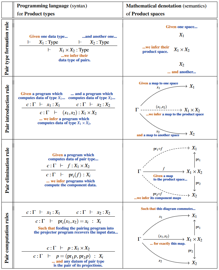
(table taken from Myers et al.)

Definition

Like any type constructor in type theory (see at natural deduction), a product type is specified by rules saying when we can introduce it as a type, how to construct terms of that type, how to use or “eliminate” terms of that type, and how to compute when we combine the constructors with the eliminators.

In natural deduction

We assume that our product types have typal conversion rules, as those are the most general of the conversion rules. Both the propositional and judgmental conversion rules imply the typal conversion rules by the structural rules for propositional and judgmental equality respectively.

The formation and introduction rules are the same for both the positive and negative product types

Formation rules for product types:

ΓAtypeΓBtypeΓA×Btype\frac{\Gamma \vdash A \; \mathrm{type} \quad \Gamma \vdash B \; \mathrm{type}}{\Gamma \vdash A \times B \; \mathrm{type}}

Introduction rules for product types:

ΓAtypeΓBtypeΓ,x:A,y:B(x,y):A×B\frac{\Gamma \vdash A \; \mathrm{type} \quad \Gamma\vdash B \; \mathrm{type}}{\Gamma, x:A, y:B \vdash (x, y):A \times B}

As a positive type

  • Elimination rules for product types:
ΓAtypeΓBtypeΓ,z:A×BCtypeΓ,x:A,y:Bc:C[(x,y)/z]Γ,z:A×Bind A×B C(c):C\frac{\Gamma \vdash A \; \mathrm{type} \quad \Gamma \vdash B \; \mathrm{type} \quad \Gamma, z:A \times B \vdash C \; \mathrm{type} \quad \Gamma, x:A, y:B \vdash c:C[(x, y)/z]}{\Gamma, z:A \times B \vdash \mathrm{ind}_{A \times B}^C(c):C}
  • Computation rules for product types:
ΓAtypeΓBtypeΓ,z:A×BCtypeΓ,x:A,y:Bc:C[(x,y)/z]Γ,x:A,y:Bβ A×B C(c):ind A×B C(c)[(x,y)/z]= C[(x,y)/z]c\frac{\Gamma \vdash A \; \mathrm{type} \quad \Gamma \vdash B \; \mathrm{type} \quad \Gamma, z:A \times B \vdash C \; \mathrm{type} \quad \Gamma, x:A, y:B \vdash c:C[(x, y)/z]}{\Gamma, x:A, y:B \vdash \beta_{A \times B}^C(c):\mathrm{ind}_{A \times B}^C(c)[(x, y)/z] =_{C[(x, y)/z]} c}
  • Uniqueness rules for product types:
ΓAtypeΓBtypeΓ,z:A×BCtypeΓ,x:A,y:Bc:C[(x,y)/z]Γ,z:A×Bu:CΓ,x:A,y:Bi (,)(u):u[(x,y)/z]= C[(x,y)/z]cΓ,z:A×Bη A×B C(c):u= Cind A×B C(c)\frac{\Gamma \vdash A \; \mathrm{type} \quad \Gamma\vdash B \; \mathrm{type} \quad \Gamma, z:A \times B \vdash C \; \mathrm{type} \quad \Gamma, x:A, y:B \vdash c:C[(x, y)/z] \quad \Gamma, z:A \times B \vdash u:C \quad \Gamma, x:A, y:B \vdash i_{(-,-)}(u):u[(x, y)/z] =_{C[(x, y)/z]} c}{\Gamma, z:A \times B \vdash \eta_{A \times B}^C(c):u =_{C} \mathrm{ind}_{A \times B}^C(c)}

Given a pointed h-proposition (A,a)(A, a), the positive product type results in (a,)(a,-) being an equivalence of types.

As a negative type

  • Elimination rules for product types:
ΓAtypeΓBtypeΓ,z:A×Bπ 1(z):AΓAtypeΓBtypeΓ,z:A×Bπ 2(z):B\frac{\Gamma \vdash A \; \mathrm{type} \quad \Gamma \vdash B \; \mathrm{type}}{\Gamma, z:A \times B \vdash \pi_1(z):A} \qquad \frac{\Gamma \vdash A \; \mathrm{type} \quad \Gamma \vdash B \; \mathrm{type}}{\Gamma, z:A \times B \vdash \pi_2(z):B}
  • Computation rules for product types:
ΓAtypeΓBtypeΓ,x:A,y:Bβ ×1(x,y):π 1((x,y))= AxΓAtypeΓBtypeΓ,x:A,y:Bβ ×2(x,y):π 2((x,y))= By\frac{\Gamma \vdash A \; \mathrm{type} \quad \Gamma\vdash B \; \mathrm{type}}{\Gamma, x:A, y:B \vdash \beta_{\times 1}(x, y):\pi_1((x, y)) =_A x} \qquad \frac{\Gamma \vdash A \; \mathrm{type} \quad \Gamma \vdash B \; \mathrm{type}}{\Gamma, x:A, y:B \vdash \beta_{\times 2}(x, y):\pi_2((x, y)) =_{B} y}
  • Uniqueness rules for product types:
ΓAtypeΓBtypeΓ,z:A×Bη ×(z):z= A×B(π 1(z),π 2(z))\frac{\Gamma \vdash A \; \mathrm{type} \quad \Gamma \vdash B \; \mathrm{type}}{\Gamma, z:A \times B \vdash \eta_{\times}(z):z =_{A \times B} (\pi_1(z), \pi_2(z))}

Given a pointed h-proposition (A,a)(A, a), the negative product type results in π 2(a,)\pi_2(a,-) being a quasi-inverse function of (a,)(a,-), rather than an equivalence of types. Thus, the positive definition is preferred to the negative definition. Alternatively, the negative product type should be defined as a coinductive type rather than an inductive type.

As a special case of the dependent sum

In dependent type theory a product type A×BA \times B is the special case the dependent sum over a:Aa : A for the special case that BB is regarded as an AA-dependent type that actually happens to be AA-independent. The rules are given as follows:

ΓAtypeΓ,x:ABtypeΓ,a:A,b:AB[a/x]B[b/x]typeΓA×Btype\frac{\Gamma \vdash A \; \mathrm{type} \quad \Gamma, x:A \vdash B \; \mathrm{type} \quad \Gamma, a:A, b:A \vdash B[a/x] \equiv B[b/x] \; \mathrm{type}}{\Gamma \vdash A \times B \; \mathrm{type}}
ΓAtypeΓ,x:ABtypeΓ,a:A,b:AB[a/x]B[b/x]typeΓA×B x:ABtype\frac{\Gamma \vdash A \; \mathrm{type} \quad \Gamma, x:A \vdash B \; \mathrm{type} \quad \Gamma, a:A, b:A \vdash B[a/x] \equiv B[b/x] \; \mathrm{type}}{\Gamma \vdash A \times B \equiv \sum_{x:A} B\; \mathrm{type}}

As a special case of the dependent product

In dependent type theory given types AA and BB, one could define a type family CC indexed by elements of the two-valued type 𝟚\mathbb{2} by C(0)AC(0) \coloneqq A and C(1)BC(1) \coloneqq B. A product type A×BA \times B is a special case of the dependent product type

A×BC(0)×C(1) x:𝟚C(x)A \times B \coloneqq C(0) \times C(1) \coloneqq \prod_{x:\mathbb{2}} C(x)

and is given by the following rules:

Formation rules for product types:

Γ,x:𝟚CtypeΓC(0)×C(1)type\frac{\Gamma, x:\mathbb{2} \vdash C \; \mathrm{type}}{\Gamma \vdash C(0) \times C(1) \; \mathrm{type}}

Introduction rules for product types:

Γ,x:𝟚c:CΓλ(x:𝟚).c(x):C(0)×C(1)\frac{\Gamma, x:\mathbb{2} \vdash c:C}{\Gamma \vdash \lambda(x:\mathbb{2}).c(x):C(0) \times C(1)}

Elimination rules for product types:

Γz:C(0)×C(1)Γp:𝟚Γz(p):C[p/x]\frac{\Gamma \vdash z:C(0) \times C(1) \quad \Gamma \vdash p:\mathbb{2}}{\Gamma \vdash z(p):C[p/x]}

Computation rules for product types:

Γ,x:𝟚c:CΓp:𝟚Γβ Π(p):λ(x:𝟚).c(x)[p/x]= C[p/x]c[p/x]\frac{\Gamma, x:\mathbb{2} \vdash c:C \quad \Gamma \vdash p:\mathbb{2}}{\Gamma \vdash \beta_\Pi(p):\lambda(x:\mathbb{2}).c(x)[p/x] =_{C[p/x]} c[p/x]}

Uniqueness rules for product types:

Γz:C(0)×C(1)Γη Π(z):z= C(0)×C(1)λ(x).z(x)\frac{\Gamma \vdash z:C(0) \times C(1)}{\Gamma \vdash \eta_\Pi(z):z =_{C(0) \times C(1)} \lambda(x).z(x)}

Properties

Suppose AA and BB are types and A×BA \times B is the negative product type of AA and BB. Then for all elements c:A×Bc:A \times B and c:A×Bc':A \times B, there is a function

ap (π 1,π 2)(c,c):(c= A×Bc)((π 1(c)= Aπ 1(c))×(π 2(c)= Bπ 2(c)))\mathrm{ap}_{(\pi_1, \pi_2)}(c, c'):(c =_{A \times B} c') \to \left((\pi_1(c) =_A \pi_1(c')) \times (\pi_2(c) =_B \pi_2(c'))\right)

There are functions ap π 1(c,c):(c= A×Bc)(π 1(c)= Aπ 1(c))\mathrm{ap}_{\pi_1}(c, c'):(c =_{A \times B} c') \to (\pi_1(c) =_A \pi_1(c')) and ap π 2(c,c):(c= A×Bc)(π 2(c)= Bπ 2(c))\mathrm{ap}_{\pi_2}(c, c'):(c =_{A \times B} c') \to (\pi_2(c) =_B \pi_2(c')) which are the function application to identities for the product projections π 1\pi_1 and π 2\pi_2, which means for all identities p:c= A×Bcp:c =_{A \times B} c', there are identities

ap π 1(c,c)(p):π 1(c)= Aπ 1(c)\mathrm{ap}_{\pi_1}(c, c')(p):\pi_1(c) =_A \pi_1(c')
ap π 2(c,c)(p):π 2(c)= Aπ 2(c)\mathrm{ap}_{\pi_2}(c, c')(p):\pi_2(c) =_A \pi_2(c')

Then, by the introduction rule for products, one could form the pair

(ap π 1(c,c)(p),ap π 2(c,c)(p))(\mathrm{ap}_{\pi_1}(c, c')(p), \mathrm{ap}_{\pi_2}(c, c')(p))

with identites

δ(c,c,p):ap (π 1,π 2)(c,c)(p)= (π 1(c)= Aπ 1(c))×(π 2(c)= Bπ 2(c))(ap π 1(c,c)(p),ap π 2(c,c)(p))\delta(c, c', p):\mathrm{ap}_{(\pi_1, \pi_2)}(c, c')(p) =_{(\pi_1(c) =_A \pi_1(c')) \times (\pi_2(c) =_B \pi_2(c'))} (\mathrm{ap}_{\pi_1}(c, c')(p), \mathrm{ap}_{\pi_2}(c, c')(p))

for all p:c= A×Bcp:c =_{A \times B} c'.

Similarly, for all elements a:Aa:A, a:Aa':A, b:Bb:B, b:Bb':B, the binary function application to identities for (,)(-, -) defined in the introduction rule for product types is given by

apbinary (,)(a,a,b,b):(a= Aa)×(b= Bb))((a,b)= A×B(a,b)\mathrm{apbinary}_{(-,-)}(a, a', b, b'):\left(a =_A a') \times (b =_B b')\right) \to ((a, b) =_{A \times B} (a', b')

inductively defined by the identities

β apbinary (,)(a,b):apbinary (,)(a,a,b,b)(refl A(a),refl B(b))= (a,b)= A×B(a,b)refl A×B((a,b)))\beta_{\mathrm{apbinary}_{(-,-)}}(a, b):\mathrm{apbinary}_{(-,-)}(a, a, b, b)(\mathrm{refl}_{A}(a), \mathrm{refl}_{B}(b)) =_{(a, b) =_{A \times B} (a, b)} \mathrm{refl}_{A \times B}((a, b)))

For all elements c:A×Bc:A \times B and c:A×Bc':A \times B, the composition of functions

apbinary (,)(π 1(c),π 1(c),π 2(c),π 2(c))ap (π 1,π 2)(c,c)\mathrm{apbinary}_{(-,-)}(\pi_1(c), \pi_1(c'), \pi_2(c), \pi_2(c')) \circ \mathrm{ap}_{(\pi_1, \pi_2)}(c, c')

has domain c= A×Bcc =_{A \times B} c' and codomain (π 1(c),π 2(c))= A×B(π 1(c),π 2(c))(\pi_1(c), \pi_2(c)) =_{A \times B} (\pi_1(c'), \pi_2(c')).

By the uniqueness rule for the negative product type, there are identities η ×(c):c= A×B(π 1(c),π 2(c))\eta_{\times}(c):c =_{A \times B} (\pi_1(c), \pi_2(c)) and η ×(c):c= A×B(π 1(c),π 2(c))\eta_{\times}(c'):c' =_{A \times B} (\pi_1(c'), \pi_2(c')), and thus, for all identities p:c= A×Bcp:c =_{A \times B} c', there are identities

c =η ×(c) (π 1(c),π 2(c)) p apbinary (,)(π 1(c),π 1(c),π 2(c),π 2(c))(ap (π 1,π 2)(c,c)(p)) c =η ×(c) (π 1(c),π 2(c)) \array{& c & \overset{\eta_{\times}(c)}= & (\pi_1(c), \pi_2(c)) & \\ p & \Vert & \rightarrow & \Vert & \mathrm{apbinary}_{(-,-)}(\pi_1(c), \pi_1(c'), \pi_2(c), \pi_2(c'))(\mathrm{ap}_{(\pi_1, \pi_2)}(c, c')(p))\\ &c' & \underset{\eta_{\times}(c')}= & (\pi_1(c'), \pi_2(c')) & \\ }

For all elements a:Aa:A, a:Aa':A, and b:Bb:B, b:Bb':B, the composition of functions

ap (π 1,π 2)((a,b),(a,b))apbinary (,)(a,a,b,b)\mathrm{ap}_{(\pi_1, \pi_2)}((a, b), (a', b')) \circ \mathrm{apbinary}_{(-,-)}(a, a', b, b')

has domain (a= Aa)×(b= Bb)(a =_A a') \times (b =_B b') and codomain (π 1((a,b))= Aπ 1((a,b)))×(π 2((a,b))= Bπ 2((a,b)))(\pi_1((a, b)) =_A \pi_1((a', b'))) \times (\pi_2((a, b)) =_B \pi_2((a', b'))).

By the computation rules of the negative product type, there are identities β ×1(a,b):π 1((a,b))= Aa\beta_{\times 1}(a, b):\pi_1((a, b)) =_A a, β ×2(a,b):π 2((a,b))= Ab\beta_{\times 2}(a, b):\pi_2((a, b)) =_A b, β ×1(a,b):π 1((a,b))= Aa\beta_{\times 1}(a', b'):\pi_1((a', b')) =_A a', and β ×2(a,b):π 2((a,b))= Ab\beta_{\times 2}(a', b'):\pi_2((a', b')) =_A b', and for all pairs of identities q:(a= Aa)×(b= Bb)q:(a =_A a') \times (b =_B b'), there are identities

π 1((a,b)) =β ×1(a,b) a π 1(ap (π 1,π 2)((a,b),(a,b))(apbinary (,)(a,a,b,b)(q))) π 1(q) π 1((a,b)) =β ×1(a,b) a \array{& \pi_1((a, b)) & \overset{\beta_{\times 1}(a, b)}= & a & \\ \pi_1(\mathrm{ap}_{(\pi_1, \pi_2)}((a, b), (a', b'))(\mathrm{apbinary}_{(-,-)}(a, a', b, b')(q))) & \Vert & \leftarrow & \Vert & \pi_1(q) \\ & \pi_1((a', b')) & \underset{\beta_{\times 1}(a', b')}= & a' & \\ }
π 2((a,b)) =β ×2(a,b) b π 2(ap (π 1,π 2)((a,b),(a,b))(apbinary (,)(a,a,b,b)(q))) π 2(q) π 2((a,b)) =β ×2(a,b) b \array{& \pi_2((a, b)) & \overset{\beta_{\times 2}(a, b)}= & b & \\ \pi_2(\mathrm{ap}_{(\pi_1, \pi_2)}((a, b), (a', b'))(\mathrm{apbinary}_{(-,-)}(a, a', b, b')(q))) & \Vert & \leftarrow & \Vert & \pi_2(q) \\ & \pi_2((a', b')) & \underset{\beta_{\times 2}(a', b')}= & b' & \\ }

Both of these square are in general not commutative squares.

In lambda-calculus

There are actually two ways to present product types, as a negative type or as a positive type. In both cases the type formation rule is the following:

A:TypeB:TypeA×B:Type \frac{A\colon Type \qquad B\colon Type}{A\times B\colon Type}

but the constructors and eliminators may be different.

As a negative type

When presented negatively, primacy is given to the eliminators. We specify that there are two ways to eliminate a term of type A×BA\times B: by projecting out the first component, or by projecting out the second.

p:A×Bπ 1p:Ap:A×Bπ 2p:B \frac{p \colon A\times B}{\pi_1 p\colon A} \qquad \frac{p\colon A\times B}{\pi_2 p\colon B}

This then determines the form of the constructors: in order to construct a term of type A×BA\times B, we have to specify what value that term should yield when all the eliminators are applied to it. In other words, we have to specify a pair of elements, one of AA (to be the value of π 1p\pi_1 p) and one of BB (to be the value of π 2p\pi_2 p).

a:Ab:B(a,b):A×B \frac{a\colon A \qquad b\colon B}{(a,b)\colon A\times B}

Finally, we have computation rules which say that the relationship between the constructors and the eliminators is as we hoped. We always have beta reduction rules

π 1(a,b) βaπ 2(a,b) βb \pi_1(a,b) \to_\beta a \qquad \pi_2(a,b) \to_\beta b

and we may or may not choose to have an eta reduction rule

(π 1p,π 2p) ηp (\pi_1 p, \pi_2 p) \to_\eta p

As a positive type

When presented positively, primacy is given to the constructors. We specify that the way to construct something of type A×BA\times B is to give something of type AA and something of type BB:

a:Ab:B(a,b):A×B \frac{a\colon A \qquad b\colon B}{(a,b)\colon A\times B}

Of course, this is the same as the constructor obtained from the negative presentation. However, the eliminator is different. Now, in order to say how to use something of type A×BA\times B, we have to specify how we should behave for all possible ways that it could have been constructed. In other words, we have to say, assuming that pp were of the form (a,b)(a,b), what we want to do. Thus we end up with the following rule:

p:A×Bx:A,y:Bc:Clet(x,y)=pinc:C \frac{p\colon A\times B \qquad x\colon A, y\colon B \vdash c\colon C}{let (x,y) = p in c \;\colon C}

We need a term cc in the context of two variables of types AA and BB, and the destructor or match “binds those variables” to the two components of pp. Note that the “ordered pair” (x,y)(x,y) in the destructor is just a part of the syntax; it is not an instance of the constructor ordered pair. In dependent type theory, this elimination rule must be generalized to allow the type CC to depend on A×BA\times B.

Now we have beta reduction rule:

let(x,y)=(a,b)inc βc[a/x,b/y] let (x,y) = (a,b) \,in c \;\to_\beta\; c[a/x, b/y]

In other words, if we build an ordered pair and then break it apart, what we get is just the things we put into it. (The notation c[a/x,b/y]c[a/x, b/y] means to substitute aa for xx and bb for yy in the term cc).

And (if we wish) the eta reduction rule, which is a little more subtle:

let(x,y)=pinc[(x,y)/z] ηc[p/z] let (x,y) = p in c[(x,y)/z] \;\to_\eta\; c[p/z]

This says that if we break something of type A×BA\times B into its components, but then we only use those two components by way of putting them back together into an ordered pair, then we might as well just not have broken it down in the first place.

Positively defined products are naturally expressed as inductive types. For instance, in Coq syntax we have

Inductive prod (A B:Type) : Type :=
| pair : A -> B -> prod A B.

(Coq then implements beta-reduction, but not eta-reduction. However, eta-equivalence is provable with the internally defined identity type, using the dependent eliminator mentioned above.)

Arguably, negatively defined products should be naturally expressed as coinductive types, but this is not exactly the case for the presentation of coinductive types used in Coq.

Positive versus negative

In ordinary “nonlinear” type theory, the positive and negative product types are equivalent. They manifestly have the same constructor, while we can define the eliminators in terms of each other as follows:

π 1p let(x,y)=pinx π 2p let(x,y)=piny let(x,y)=pinc c[π 1p/x,π 2p/y] \begin{aligned} \pi_1 p &\;\coloneqq\; let (x,y) = p in x\\ \pi_2 p &\;\coloneqq\; let (x,y) = p in y\\ let (x,y) = p in c &\;\coloneqq\; c[\pi_1 p / x, \pi_2 p / y] \end{aligned}

It is obvious that the β\beta-reduction rules in the two cases correspond; see below for η\eta-conversion.

In dependent type theory, in order to recover the dependent eliminator for the positive product type from the eliminators for the negative product type, we need the latter to satisfy the η\eta-conversion rule so as to make the above definition well-typed. It is sufficient to have the η\eta-conversion up to propositional equality, however, if we are willing to insert a substitution along such an equality in the definition of the dependent eliminator. Conversely, the dependent eliminator for the positive product allows us to prove a propositional version of the negative η\eta-conversion (without assuming the positive η\eta-conversion). See propositional eta-conversions.

Now from η\eta-conversion for the negative product, we can also derive

let(x,y)=pinc[(x,y)/z] c[(π 1p,π 2p)/z] ηc[p/z] \begin{aligned} let (x,y) = p in c[(x,y)/z] &\;\coloneqq\; c[(\pi_1 p,\pi_2 p)/z]\\ &\;\to_\eta\; c[p/z] \end{aligned}

so the defined positive product also satisfies its η\eta-conversion, which will be definitional or propositional according to that of the negative product.

On the other hand, if the positive product has a definitional η\eta-conversion, then for the defined negative product we have

(π 1p,π 2p) (let(x,y)=pinx,let(x,y)=piny) η(let(x,y)=pin(let(x,y)=(x,y)inx,let(x,y)=(x,y)iny) βlet(x,y)=pin(x,y) ηp \begin{aligned} (\pi_1 p, \pi_2 p) &\;\coloneqq\; (let (x,y) = p in x, let (x,y) = p in y)\\ &\;\leftarrow_\eta\; (let (x',y') = p in \;( let (x,y) = (x',y') in x , let (x,y) = (x',y') in y )\\ &\;\to_\beta\; let (x',y') = p in (x',y')\\ &\;\to_\eta\; p \end{aligned}

Note that this involves a beta-reduction step and also a “backwards” η\eta-reduction step. So from positive η\eta reduction we cannot derive negative η\eta-reduction, only negative η\eta-equivalence. (However, the directionality of η\eta-reduction is somewhat questionable anyway.)

In conclusion, we have:

  • In non-dependent type theory, positive and negative products are equivalent, as are their definitional β\beta-reduction rules.

  • In dependent type theory with identity types, improving the positive eliminator to a dependent eliminator is equivalent to asserting propositional versions of either η\eta-conversion rule.

  • In any case, the two definitional η\eta-conversion rules also correspond.

It is of importance to note that these translations require the contraction rule and the weakening rule; that is, they duplicate and discard terms. In linear logic these rules are disallowed, and therefore the positive and negative products become different. The positive product becomes “tensor” ABA\otimes B, and the negative product becomes “with” A&BA \& B.

Categorical interpretation

Under categorical semantics, product types satisfying both beta and eta conversions correspond to products in a category. More precisely:

  • categorical products may be used to interpret product types that validate both beta and eta rules, while

  • the syntactic category of a type theory with product types has categorical products, as long as the type theory satisfies both beta and eta rules.

Of course, the categorical notion of product matches the negative definition of a product most directly. In linear logic, therefore, the categorical product interprets “with” &\&, while an additional monoidal structure interprets “tensor” \otimes. On the other hand, in a representable cartesian multicategory, the product has a “from the left” universal property which matches the positive definition.

There is also another interpretation in category theory of the product type AA and BB, as the initial AA-indexed family of parallel morphisms with source BB, the object A×BA \times B with a family of morphisms

in A(x):BA×B\mathrm{in}_A(x):B \to A \times B

such that for any other object CC with a family of morphisms f(x):BCf(x):B \to C, there exists a unique morphism u C:A×BCu_C:A \times B \to C such that

u Cin A(x)=f(x)u_C \circ \mathrm{in}_A(x) = f(x)

This corresponds to the positive product types.

References

A textbook account in the context of programming languages is in section 11 of

On product types as inductive types:

  • Kajetan Söhnen, §2.4.3 in : Higher Inductive Types in Homotopy Type Theory, Munich (2018) [pdf, pdf]

Last revised on January 1, 2024 at 04:05:20. See the history of this page for a list of all contributions to it.