nLab infinitesimal object
Context
Formal geometry
Synthetic differential geometry
synthetic differential geometry
Introductions
from point-set topology to differentiable manifolds
geometry of physics: coordinate systems, smooth spaces, manifolds, smooth homotopy types, supergeometry
Differentials
Tangency
The magic algebraic facts
Theorems
Axiomatics
Models
differential equations, variational calculus
Chern-Weil theory, ∞-Chern-Weil theory
Cartan geometry (super, higher)
Compact objects
Contents
- Idea
- Formalization in synthetic differential geometry
- Realizations in algebraic geometry
- Comparison to infinitesimals in nonstandard analysis
- Definition
- Examples
- Infinitesimal intervals
- The standard infinitesimal interval
- The cartesian product of infinitesimal intervals
- The -dimensional infinitesimal disk
- The infinitesimal neighbourhood
- Spaces of infinitesimal -simplices
- Related concepts
- References
Idea
An infinitesimal quantity is supposed to be a quantity that is infinitely small in size, yet not necessarily perfectly small (zero). An infinitesimal space is supposed to be a space whose extension is infinitely small, yet not necessarily perfectly small (pointlike).
Infinitesimal objects have been conceived and used in one way or other for a long time, notably in algebraic geometry, where Grothendieck emphasized the now familiar role of formal duals (affine schemes) of commutative rings with nilpotent ideals as infinitesimal thickenings of the formal dual of the quotient ring .
See also infinitesimally thickened point.
Formalization in synthetic differential geometry
A proposal for formalizing the abstract nonsense behind the notion of the infinitesimal such that these algebraic constructions become models for more general axioms was given by William Lawvere in his 1967 lecture (see the references below).
Lawvere observed that a simple yet powerful characterization of the notion of infinitesimal space is that is an object in a topos of spaces such that the inner hom functor has a right adjoint.
If the topos in question furthermore is equipped with a line object that plays the role of the real line then a sensible notion of infinitesimal quantities in is obtained when all morphisms from infinitesimal spaces are necessarily linear maps. This is now known as the Kock-Lawvere axiom on lined toposes . When it is satisfied, is called a smooth topos. The study of these is known as synthetic differential geometry.
The notion of infinitesimal object and infinitesimal space then makes sense in any smooth topos, and may be reasoned about generally for all smooth toposes. In any concrete model for the axioms there will accordingly be concrete realizations of these infinitesimal objects.
Realizations in algebraic geometry
Notably, for instance the Grothendieck topos of presheaves on the opposite category of that of commutative -algebras (over some field ) is a simple realization of a smooth topos (see for instance Kock-SGM, section 93). This topos and its variants and in particular their sheaf-localizations provide the context in which algebraic geometry takes place.
Therefore the notion of infinitesimals in algebraic geometry may be understood as being models of the general notion of infinitesimals in synthetic differential geometry in context such as or similar.
The vast majority of existing work on infinitesimals and infinitesimal neighbourhoods comes from algebraic geometry. It is the foundation of Grothendieck’s approach to regular differential operators, to costratifications, crystalline cohomology and de Rham descent.
Similar infinitesimal thickenings also appear in the noncommutative geometry of Kapranov, and in the language of abelian categories of quasicoherent sheaves in the work of Lunts and Rosenberg on regular differential operators in the content of noncommutative geometry, which strongly takes into account tensor products.
Comparison to infinitesimals in nonstandard analysis
Another notion of infinitesimals has arisen in the context of nonstandard analysis. The infinitesimal quantities considered there differ from the general ones in synthetic differential geometry in that they are all invertible (their inverses being “infinitely large”). Nevertheless, one can construct models of synthetic differential geometry which, in addition to nilpotent infinitesimals, contain invertible infinitesimals; see for instance MSIA, chapters VI and VII. Such invertible infinitesimals can be applied in some of the same ways as the infinitesimals of nonstandard analysis.
However, as pointed out in MSIA (intro. to Chapter VII), “there are some obvious differences.” The primary tool used in nonstandard analysis is a completely general transfer principle, saying that any statement in the ordinary world is also true in the nonstandard world. In particular, this implies that the infinitesimal and infinitely large quantities in nonstandard analysis obey all the same rules of arithmetic and analysis as do the standard ones. By contrast, a limited sort of transfer principle relating a pair of specific models for SDG is proven in MSIA, but it applies only to statements of a certain logical form. Moreover, the arithmetic of invertible infinitesimals in SDG has some unfamiliar aspects: for instance, mathematical induction is only valid for statements of a certain logical form, and the axiom of finite choice fails.
The construction of models for nonstandard analysis does, however, have a topos-theoretic description, using filterpower?s.
Definition
Atomic object
Definition (Lawvere)
In a cartesian closed category an object is called infinitesimal atomic if the hom-functor for maps out of (i.e. the functor of exponentiation by ) is a left adjoint, i.e. if it has a right adjoint.
An object which is infinitesimal atomic is small from the internal perspective of the category. In contrast, an object is a tiny object when it is small from the external perspective, that is when the functor into the category of sets preseves colimits.
When is a local Grothendieck topos over , then the two notions agree, but they do not in general. For example the terminal object in is always internally small (infinitesimal atomic), since the functor always has a right adjoint. But it is not necessarily a tiny object from the external perspective, since need not preserve colimits. This happens in situations where it is not appropriate to view the terminal object in a categoy as a small object from the external perspective, for example when we are in a slice topos . In such cases the correct intuitive external meaning of an object being internally small is that it is small in each fiber.
Remark
(intuitive interpretation)
Here is how to think of what this definition means intuitively. For that, notice how maps out of an ordinary space fail to preserve colimits:
for definiteness, consider the case of a cover of a space by spaces so that is the coequalizer
as discussed in detail at sieve and sheaf. This says effectively that every point of is element of at least one of the covering spaces and that one obtains by identifying the points in the covering spaces that correspond to the same one in .
Now let be any other space. We may assume here that the internal hom at least preserves coproducts, so that applying this functor to the above diagram yields
Now notice how this will in general fail to still be a coequalizer: if it were, for one the morphism would have to be an epimorphism. But this can’t be in general, because it would mean that every map factors through one of the covering spaces. The problem here is that in general the image of may be larger than any of the .
This is maybe most familiar in the context of loop spaces (for the circle): the loop space of a cover of is not in general a cover of the loop space.
But suppose that were infinitesimal. One thing that should mean is that there is no other space that is “effectively smaller” in some useful sense. For infinitesimal, we do expect that every map can always be factored through at least one of the : because is so small, the image of a map out of it can never be too large.
So only if qualifies as having infinitesimal extension can the functor be expected to preserve colimits.
Formal infinitesimal space
Definition (formal infinitesimal space)
An object in a smooth topos is called a formally infinitesimal object if it is the algebra-spectrum of (what in the sdg-literature is usually called) a --Weil algebra in
Here
-
is an internal -algebra object in with an -finite dimensional nilpotent ideal
-
is the subobject of the internal hom of morphisms that respect the -algebra structure on and .
All the spaces that are described as collection of degree infinitesimal neighbours are of this form. Infinitesimal spaces not of this form are germ-spaces (see the examples below). These violate the finite-dimensionality assumption on .
Examples
Infinitesimal intervals
There are several different objects that one may think of as an infinitesimal interval.
The smallest of them is often denoted and sometimes called the disembodied tangent vector or the walking tangent vector .
This is described in more detail at
It is such that a morphism into a manifold is the same as a choice of point and of a tangent vector . Equivalently, it is such that restricting a smooth function along the inclusion produces the first-order jet defined by at the point .
Accordingly, for each there is a “slightly bigger” infinitesimal interval often denoted , which is such that restricting a smooth function along produces the order- jet represented by this function at the given point.
Still infinitesimal but bigger than all these is the object of intersections of all neighbourhods of the origin of . This is such that the restriction of a map along produces the germ of at .
The standard infinitesimal interval
Models
The classical example of a realization of an infinitesimal object is in terms of what is (traditionally but undescriptively) called the ring of dual numbers. For that we place ourselves in some context in which spaces are characterized dually in terms of the quantities on them, i.e. in terms of their would-be function algebras.
For some real number , functions on the closed interval of length may be thought of as represented by functions on the whole real line , where two representatives represent the same function on the interval if they differ by a function that vanishes on the interval.
Precisely:
Lemma
The (generalized smooth) algebra of smooth functions on is isomorphic to the quotient of the algebra of smooth functions on all of by the functions that vanish on
Proof
This is a corollary of the smooth version of the Tietze extension theorem, which says that for a closed subset, every smooth function on extends to a smooth function on all of .
See page 20 of MSIA.
As we think of the length of the interval shrinking to an infinitesimal value, the notion of derivative of functions is such that we want to say that the statement “a function vanishes on the infinitesimal interval” is equivalent to “a function vanishes at the origin and its first derivative there vanishes, too”. This in turn is usually equivalent (in a smooth context) to “a function is a square of a function that vanishes at the origin”.
Accordingly, in a context where one considers polynomial functions over the ground field , the infinitesimal interval is given by the space – usually called – that is dual to the ring which is the quotient of the polynomial ring in one variable modulo the polynomial . This is often called the ring of dual numbers (where the term ‘dual’ historically refers to its being -dimensional). In terms of generators and relations this is the ring generated by a single element subject to the relation that .
Similarly, in the smooth context of, for instance, Moerdijk–Reyes Models for Smooth Infinitesimal Analysis, is the space dual to the generalized smooth algebra obtained as the smooth functions on the real line modulo squares of functions that vanish at the origin.
Definition (the 1-dimensional infinitesimal space)
In the context of generalized smooth algebra, the -dimensional infinitesimal space is the space whose function algebra is the quotient
of all functions on the real line, modulo those that are a product with the function .
This does reproduce the above ring of dual numbers due to the Hadamard lemma, which says that for a smooth function, there exists a smooth function such that for all we have . So modulo , every smooth function is in fact a polynomial function.
See pages 19-20 of MSIA.
In this dual generators-and-relations description, the infinitesimal interval is very familiar in many mathematically less sophisticated contexts. It prevails for instance in the basic physics textbook treatment since Isaac Newton up to this day. Sophus Lie is famously quoted as having said that he found many of his famous insights by such “synthetic reasoning” and only a lack of proper formalization prevented him from writing them up in this way instead of in the more wide-spread way of differential calculus.
Axiomatics
More generally, one may abstract the above properties of concrete realizations of the infinitesimal interval such as to get such a notion in an arbitrary suitable context. A suitable context for synthetic differential geometry is any topos equipped with an internal commutative ring .
Using the topos-internal logic we may speak of both and as if they were sets, where “element” means generalized element. This way we have:
Example
Let be a smooth topos. Then the first order infinitesimal interval object is the subobject of of all those elements whose square is 0.
It may be helpful to recall that in terms of limits this notation means that is the equalizer of
and
For with any morphism embodying a generalized element , the universal property of the limit identifies this uniquely with a morphism , hence with a generalized element of , such that is the element of with domain of definition : .
The cartesian product of infinitesimal intervals
This works analogously to how the -cube is the -fold cartesian product of the unit interval with itself.
Example
The -fold cartesian product of the first-order infinitesimal interval , example , with itself might be called the “infinitesimal -cube”.
By the discussion at smooth algebra, we have
The -dimensional infinitesimal disk
Example
For the -dimensional infinitesimal disk is
Remark
Since in particular for all elements of the infinitesimal -disk, we have an inclusion
which is proper if . For we have .
While is closed under multiplication by elements of , it is not in general closed under addition of its elements. For instance for we have that (the operation being in ) is still in precisely if is in .
The infinitesimal neighbourhood
For a point in a manifold, the infinitesimal neighbourhood is the intersection of all open neighbourhoods of . This is such that the restriction of a function along the inclusion is precisely the “infinitesimal germ” of the function .
All of the infinitesimal spaces above are contained in the corresponding infinitesimal neighbourhood. So this is the “largest” of the infinitesimal spaces discussed here.
Spaces of infinitesimal -simplices
Much of this is being reworked at infinity-Lie algebroid.
Idea
An infinitesimal -simplex in based at the origin is a collection of points in , such that each is an infinitesimal neighbour of the origin
and each are infinitesimal neighbours of each other
Following section 1.2 of
- Anders Kock, Synthetic differential geometry of manifolds (pdf)
we write for the space of all infinitesimal -simplices in . More precisely, this is defined as the formal dual of the algebra defined as follows.
Functions on spaces of infinitesimal -simplices turn out to be degree -differential forms. This provides a “synthetic” way of precisely thinking of wedge produts etc as products of infinitesimals. As the following computations do show, the skew-commutativity of the wedge product is an inherent consequence of the nature of infinitesimals.
Definition
Definition
The algebra is the commutative -algebra generated from generators subject to the relations
and
Remark
By multiplying out the latter set of relations and using the former, these relations are seen to be equivalent to the set of relations
Notice that this implies also that
A general element of this algebra we think of as a function on a certain infinitesimal neightbourhood of the origin of , interpreted as the space of infinitesimal -simplices in based at 0.
Since is a Weil algebra in the sense of synthetic differential geometry, its structure as an -algebra extends uniquely to the structure of a smooth algebra (as discussed there) and we may think of as an infinitesimal smooth locus.
Example
For and we have that consists of elements of the form
for and a collection of ordinary covectors and with “” denoting the evident contraction, and where in the last step we used the above relations.
It is noteworthy here that the coefficient of the term which is multilinear in each of the is the wedge product of two covectors and : we may naturally identify the subspace of on those elements that vanish if either or are set to 0 as the space of 2-forms at the origin of .
Of course for this identification to be more than a coincidence we need that this is the beginning of a pattern that holds more generally. But this is indeed the case.
Properties
Let be the set of square submatrices of the -matrix . As a set this is isomorphic to the set of pairs of subsets of the same size of and , respectively. For instance the square submatrix labeled by and is
For an submatrix, we write
for the corresponding determinant, given as a product of generators in . Here the sum runs over all permutations of and is the signature of the permutation .
Proposition
The elements are precisely of the form
for unique . In other words, the map of vector spaces
given by
is an isomorphism.
Proof
This is a direct extension of the argument in the above example: a general product of generators in is
By the relations in , this is non-vanishing precisely if none of the -indices repeats and none of the -indices repeats. Furthermore by the relations, for any permutation of elements, this is equal to
It follows that each such element may be written as
where is the subdetermined given by the subset and as discussed above.
Remark
In section 1.3 of
- Anders Kock, Synthetic differential geometry of manifold (pdf)
effectively this proposition appears as the “Kock-Lawvere axiom scheme for ” when is regarded as an object of a suitable smooth topos. It is useful to record this simple but very crucial observation of Anders Kock here in the category or in the category of smooth loci, as we do here, where it is just a simple observation. The point of the Kock-Lawvere axiom scheme is effectively to ensure that the properties of are preserved under Yoneda embedding into a corresponding sheaf topos. But it has been observed that it serves to clarify what is going on in parts of Ander Kock’s book by separating the combinatorial and algebraic arguments from their internalization into suitable smooth toposes.
Let be the sub-vector space of the underlying vector space of on those elements that vanish if the collection of generators is set to 0, for all . This are those elements that are linear combinations of the form , for ranging over the maximal square submatrices of .
So inside the space of functions on infinitesimal simplices, we find the differential forms. The next crucial observation now is that there is a natural reason , from the nPOV, to restrict to .
The tangent Lie algebroid and differential forms
The collection of the spaces for all naturally forms a simplicial smooth locus , which represents the infinitesimal path ∞-groupoid? of , equivalently the tangent Lie algebroid of .
Dually this is a smooth cosimplicial algebra. Under the normalized cochain complex functor of the dual Dold-Kan correspondence this identifies with a dg-algebra. The fact that this is the normalized cochain complex algebra means that it consists in degree only of a subspace of the space that the cosimplicial algebra has in degree . This subspace is precisely that of differential -forms.
This we now describe in detail. All the arguments involved are still (with slightly different parameterization, possibly) due to Anders Kock, the only new thing here being the observation that the restriction to the joint kernel of the degeneracy maps exhibts the Dold-Kan map, and that this way using the simplicial picture everything acquires a nice nPOV interpretation as being about the infinitesimal path ∞-groupoid? of , regarded either as an infinitesimal Lie ∞-groupoid or as a ∞-Lie algebroid.
Definition
Consider the simplicial smooth locus
where
-
the face maps are
-
for given by
-
for given by
-
for given by
-
-
the degeneracy maps are
Dually (and this may be taken now as the precise definition of what the above simplicial object is), this is the smooth cosimplicial algebra
where
-
the co-degeneracy maps are given on generators by
-
for sending to itself regarded as an element of ;
-
for sending to 0;
-
for sending to .
-
-
the co-face maps are given on generators
-
for by sending
, , , , ;
-
for by sending each to the generator of the same name;
-
for by sending
where is obtained from by replacing each it contains with .
-
The way to think of how the face and degeracy maps here work is to imagine that a collection of elements spans an infinitesimal -parallelepiped, and that inside that the face and degeneracy maps slice out a -simplex. The proof that this is indeed a (co)simplicial object is entirely analogous to the discussion of the simplicial object of finite simplices at interval object.
For instance for we have six 3-simplices sitting inside each 3-cube
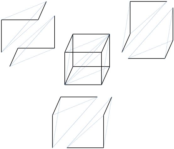
and the face maps identify one of these:
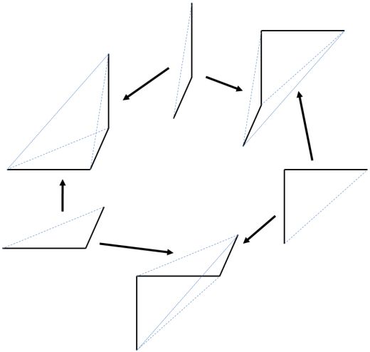 .
.
Now observe that under the dual Dold-Kan correspondence the normalized cochain complex of this cosimplicial algebra is, up to isomorphism, the complex that in degree has the joint kernel of the co-degeneracy maps. But by the above remarks, this joint kernel is precisely
the space of differential -forms on .
Theorem
The normalized cochain complex of the cosimplicial algebra is isomorphic as a cochain complex to the de Rham complex of .
Equipped with the cup product induced from is is isomorphic to the de Rham complex even as a dg-algebra.
Proof
We have already seen that degreewise the vector spaces in question are isomorphic.
It remains to check that the differentials agree. The alternating sum of the face maps acts on an element
as
Under our identification this means that the alternating sum of the face maps sends
where each is a constant 1-form on . So this is indeed the action of the de Rham differential.
The construction of is manifestly natural and extends to a functor
from CartSp to simplicial smooth loci. Effectively just by (derived) Yoneda extension of this functor to a functor on simplicial presheaves on CartSp one obtains a definition of the infinitesimal path ∞-groupoid? of any smooth manifold, any diffeological space and even every ∞-Lie groupoid.
Related concepts
Examples of sequences of local structures
References
Discussion of infinitesimals goes back to Leibniz.
- Hermann Cohen, Das Prinzip der Infinitesimal-Methode und seine Geschichte , Berlin 1883. (html)
Nowadays infinitesimal spaces and their properties were familiar in all those areas of mathematics where spaces are characterized by the algebras of functions on them.
It was in a seminal lecture
- William Lawvere, Categorical Dynamics lectures at the University of Chicago (1967)
reproduced in
- Anders Kock, Topos theoretic methods in Geometry, Aarhus Universitet (1979)
that the proposal was made to axiomatize the properties of infinitesimal objects by making use of the fact that they are supposed to be objects of a cartesian closed category.
It was from this insight that synthetic differential geometry was eventually developed.
- William Lawvere, Outline of synthetic differential geometry,
(web)
This is a classical case of general abstract nonsense used to understand a subtle situation.
A summary and discussion of the axiomatically defined standard infinitesimal objects , , is in section 1.2 of
- Anders Kock, Synthetic Geometry of Manifolds (pdf)
Atomic spaces
The proposal to call objects such that has an amazing right adjoint “atomic objects” is due to
- William Lawvere, Toposes of Laws of Motion
and repeated in
- William Lawvere, Open problems in topos theory (pdf)
Details on the right adjoint to the exponentiation functor for an infinitesimal object are in appendix 4 of
- Moerdijk, Reyes, Models for Smooth Infinitesimal Analysis
Formally infinitesimal spaces
For formal infinitesimal objects and Weil algebras see
section I.16 of
- Anders Kock, Synthetic differential geometry (pdf)
and chapter I, section 4 and chapter II, theorem 1.13 and onwards in
A discussion on terminology and share of the content between infinitesimal object and infinitesimal quantity is saved at Forum here.
For an approach to infinitesimal thickenings in the context of abelian categories of quasicoherent sheaves see differential monad and regular differential operator in noncommutative geometry.
Last revised on March 5, 2023 at 10:29:22. See the history of this page for a list of all contributions to it.