nLab fundamental (infinity,1)-category
Context
-Category theory
Background
Basic concepts
-
equivalences in/of -categories
Universal constructions
Local presentation
Theorems
Extra stuff, structure, properties
Models
Homotopy theory
homotopy theory, (∞,1)-category theory, homotopy type theory
flavors: stable, equivariant, rational, p-adic, proper, geometric, cohesive, directed…
models: topological, simplicial, localic, …
see also algebraic topology
Introductions
Definitions
Paths and cylinders
Homotopy groups
Basic facts
Theorems
Contents
Idea
In analogy to how a topological space has a fundamental ∞-groupoid, a directed space has a fundamental (∞,1)-category
Definition
Directed topological spaces
Definition
By a directed topological space we here mean specifically a pair consisting of
-
a subset of continuous maps that are are labeled as being directed ,
-
such that
-
for every orientation preserving homeomorphism and every directed map also is directed;
-
for any two directed paths with also the concatenation
is a directed path.
-
A morphism of directed spaces is a continuous map that takes elements in to elements in .
This defines the category of directed topological spaces.
Example
(topological poset)
For a topological space equipped with the structure of a poset on its underlying set, say that is directed if for all in we have in .
Example
(directed geometric simplex)
For the standard topological -simplex its standard directed paths are order-preserving maps into its 1-skeleton (the union of the 1-faces equipped with the evident poset-structure induced from that on the vertices), such that the endpoints land on vertices.
Example
(directed geometric realization)
For a quasi-category its geometric realization becomes a directed topological space by taking the directed paths to be all maps that factor through its 1-skeleton:
while preserving the canonical order and so that the endpoints land on vertices.
The previous example of the directed topological simplex is the special case of this for .
Fundamental -category
Definition
The fundamental -category of a directed topological space is given by the quasi-category whose k-morphisms are those continuous maps
that are morphisms of directed spaces with respect to the standard directed paths in .
Lemma
This does indeed define a quasi-category
Proof
Use the standard retracts of the topological horn inclusions to fill horns in .
For these retracts are the identity on 1-faces, hence trivially preserve the directed paths. For it is precisely the retract of the inner horn that preserves the directed paths. This is sufficient to satisfy the inner horn filler condition of quasi-categories.
Properties
Observation
If is undirected in that all paths are labeled as directed – – then coincides with the fundamental ∞-groupoid of .
Fundamental -categories induced from intervals
The interest in interval objects is that various further structures of interest may be built up from them. In particular, since picking an interval object is like picking a notion of path, in a category with interval object there is, under mild assumptions, for each object an infinity-category – the fundamental -category of with respect to – whose k-morphisms are -fold -paths in .
There are different ways to make this precise and realize it in detail. The main distinction is whether one uses
or
We describe an algebraic version in terms of Trimble omega-categories and then a geometric version in terms of cubical objects and simplicial objects.
Fundamental algebraic -categories
The collection of objects in a category with interval object naturally comes equipped with the structure of an operad: this is the tautological co-endomorphism operad on the object in the symmetric closed monoidal category of bi-pointed objects from to .
This induces in turn for all objects on the object the structure of an operad, which is naturally interpreted as an internal -category structure on
This internal -category is denoted
and interpreted as the fundamental groupoid or rather, in general, the fundamental category of the object with respect to the interval object – all internal to .
Moreover, by iterating this process as described at Trimble n-category one should obtain, if everything goes through, on the structure of a Trimble -category and indeed a functor
(… to be continued …)
Remarks
-
The condition that all are contractible is the coherence condition on all composition operations.
-
The above is not demanding that the interval object itself is is weakly equivalent to the point. If it is, then is indeed a fundamental groupoid. If it is not, then may just be a fundamental category.
-
If has a notion of path object one may consider imposing the condition that is a path object of for all . Similarly, if has a cylinder functor, one may consider imposing the condition that it is given by .
Fundamental geometric -categories
Let be a category with finite limits and (plain) interval object , where denotes the terminal object.
This may or may not come with further structures and properties as discussed in the definitions above. For the following however no more than that is neceesray.
Recall that the cube category is the initial strict monoidal category equipped with an object together with two maps and a map such that .
In a tautological way, induces a cocubical object in , a functor
from the cube category to . This sends the abstract interval object that the cube category is freely generated from to the given , and sends to the -cuber .
For every object homming cubes into thereby produces a cubical set
One tends to want to regard this as the cubical incarnation of the fundamental -category of with respect to the notion of path given by .
However, while cubes are nice for many purposes, it is a sad fact of life that the homotopy theory for cubical structures (while certainly it does exist in full beauty in principle) is much less well developed to date (maybe that will change in the future) than that of simplicial structures. For many purposes in higher category theory, therefore, it will be useful to take a slightly different perspective on , without essentially changing it.
In fact, there is also naturally the structure of a cosimplicial object of the collection of -cubes. This differs from the cubical structure only in were precisely one injects the boundaries into an
Definition (cosimplicial object induced from interval object)
Given a cartesian interval object , define a cosimplicial object
as follows:
-
the object in degree is the -fold product of with itself:
-
the degeneracy map is given by projecting out the -factor:
-
the face map is given
-
for by inserting in the -factor:
-
for by inserting in the -factor:
-
for by duplicating the -factor:
-
Proposition
The maps defined this way indeed satisfy the simplicial identities.
Proof
This is straightforward to check, if a little tedious due to the many case distinctions.
Remark (unwrapping the definition)
It may be helpful to unpack the above definition a bit.
Remark
(collars)
This construction gives “collared simplices” in much the same sense as in collared cobordism and in A1-homotopy:
there is no condition that the morphisms “hit a boundary point” – whatever that may mean in – of . For instance in a lined topos is canonically chosen to be the given line object and will hence typically “extended indefinitely” beyond these points.
An example of this in practice is the A1-homotopy theory of schemes – there is no exact analogue of the interval (with boundary points) in an algebraic setting, but the affine line together with the canonical points 0 and 1 is an interval object.
So need not “look” much like a 1-simplex, but the choice of boundary points and allows us to regard it as an interval for all practical purposes.
Similarly and more generally what the above construction manifestly defines are cubes built from . But then the simplicial choice of boundaries inside these cubes allows to think of them as just the simplices “sitting inside” these cubes.
All these statement become precise for specific typical choices of the ambient category , discussed in the examples below.
An important aspect is that once the cosimplicial object of collared simplices is used to form simplicial objects (discussed below) and when these are interpreted as models for ∞-groupoids, then the collars disappear: they are part of the model, but, roughly, don’t affect the equivalence class of the object that this model models.
For instance with used as the interval in Top, a path in a topological space is an entire curve , but two such paths are composable already when , irrsepctive of how extends and irrsepctive of how extends .
Moreover, the composite-up-to-homotopy of these two paths is an entire surface in , but what only matters for this surface qualifying as a compositor of is that its -segment and its segment coincide with the corresponding segments in and .
More on this in the following example section.
Example: standard intervals, cubes and simplices in and
Let Top or Diff be the category of topological spaces or of manifolds.
A standard choice of interval object in is with the obvious two boundary inclusions .
But another possible choice is to let be the whole real line, but still equipped with the two maps , that hit the and , respectively.
Either of these two examples will do in the following discussion. The second choice is to be thought of as obtained from the first choice by adding “infinitely wide collars” at both boundaries of . While may seem like a more natural choice for a representative of the idea of the “standard interval”, the choice is actually more useful for many abstract nonsense constructions.
But since it is hard to draw the full real line, in the following we depict the situation for the choice .
Then for low the above construction yields this
-
– here is the point.
-
– here is just the interval itself
The two face maps and pick the boundary points in the obvious way. The unique degeneracy map maps all points of the interval to the single point of the point.
-
– here is the standard square
But the three face maps of the cosimplicial object constructed above don’t regard the full square here, but just a triangle sitting inside it, in that pictorially they identify -shaped boundaries in as follows:
(here the arrows do not depict morphisms, but the standard topological interval, i don’t know how to typeset just lines without arrow heads in this fashion!)
-
– here is the standard cube
Exercise
Insert the analog of the above discussion here and upload a nice graphics that shows the standard cube and how the cosimplicial object picks a solid tetrahedron inside it.
As a start, we can illustrate how there are 6 3-simplices sitting inside each 3-cube.
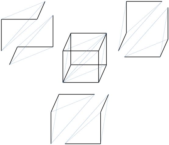
Once you see how the 3-simplices sit inside the 3-cube, the facemaps can be illustrated as follows:
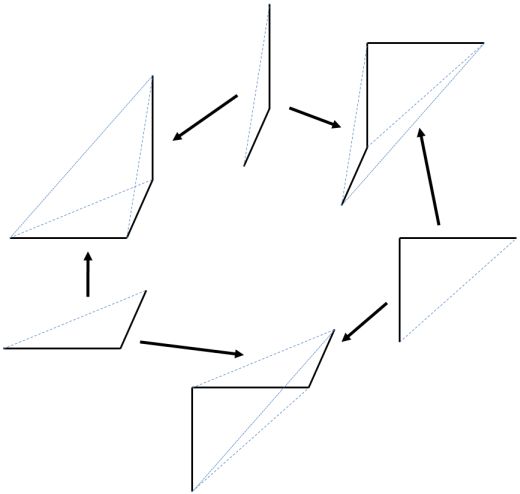
Note that these face maps are to be thought of as maps into 3-simplices sitting inside a 3-cube.
Fundamental little 1-cubes space induced from an interval
Urs Schreiber: something I am thinking about…
The following is supposed to give an (∞,1)-operadic incarnation of the notion of fundamental -groupoid induced from an interval object. It should resemble a geometric operadic version of the algebraic operadic version described further above.
Let be the category of planar trees, so that a presheaf on is a planar dendroidal set.
Given an interval object in a category , assume one isomorphism for each has been chosen.
Then there is a planar co-dendroidal object in given by:
-
a tree with leaves is sent to
(we think of the -th copy of here as being associated to the th leaf of the planar tree);
-
every degeneracy map is sent to the corresponding identity morphism
(this corresponds to the fact that the co-dendroidal object encodes no nontrivial unary (co)operations, only the -ary operations encoded nontrivial infomation);
-
an outer face map on an -ary vertex is the identity on all copies of corresponding to the unaffected leaves and is on the affected leaf;
-
an inner face map that contracts a -ary vertex with a -ary one is the identity on all unaffected leaves and is on the affected leaves the composition
Example. In Top with the standard interval, and let be the map given by multiplication of real numbers by .
Then for the planar tree given by
the inclusion of the tree into given by identifying it with its root is sent to the map that is the composite of the map wth the map that is multiplication by two on and addition by 1 on .
On the other hand the inner face map from
to corresponds to the map that is the composite of the map with the above map .
Now for any object, we obtain the planar dendroidal set
It assigns to any tree with leaves the hom-set . This we can think of as the set of standard parameterized paths of parameter length in . The action of tree morphisms on these sets is the reparameterization of these paths as encoded in the tree structure.
In particular, we have the dendroidal set of the interval object itself. This is something like the little 1-cubes operad as seen by .
I think for every there is an evident morphism of dendroidal sets
The component over the tree sends all of to ….
For a pointed object, there is the sub-dendroidal set of paths whose endpoints map to the basepoint.
Related concepts
-
fundamental category, fundamental -category
References
The above definition, evident as it may be, does not seem to be in the literature. Articles that do discuss proposals for aspects of fundamental higher categories of directed spaces include
-
Marco Grandis, Directed homotopy theory, I. The fundamental category (arXiv)
-
Tim Porter, Enriched categories and models for spaces of evolving states, Theoretical Computer Science, 405, (2008), pp. 88–100.
-
Tim Porter, Enriched categories and models for spaces of
dipaths. A discussion document and overview of some techniques_ (pdf)
The simplicially enriched categories obtained from a directed space according to the latter have as morphisms directed paths, and as 2-morphisms directed homotopies (paths of directed paths). This is in contrast to the above definition, where the 2-cells away from their boundary are unconstrained.
Accordingly it seems that the definition by Porter produces indeed not a Kan-complex enriched category (a model for an -category) but a quasi-category-enriched category, hence actually a model for an (∞,2)-categories, a candidate for the fundamental -category of a space. Generally, in the fundamental (∞,n)-category the -cells should be directed maps, and the -cells be otherwise unconstrained.
Last revised on June 17, 2019 at 11:50:36. See the history of this page for a list of all contributions to it.