Schreiber Super Lie n-algebra of Super p-branes

The following are a couple of related talks that I have given.

Expository talk notes are below. For more detailed lecture notes see: geometry of physics – fundamental super p-branes. For related talk notes see Super p-Brane Theory emerging from Super Homotopy Theory and Super topological T-Duality.

• Urs Schreiber,

  Super Lie $n$-algebra of Super $p$-branes

  talks at

  Fields, Strings, and Geometry Seminar, Surrey, 5th-9th Dec. 2016

  Abstract. It is “well known” that the Green-Schwarz sigma models for the superstring and the membrane are higher super-WZW-type models classified by super Lie algebra cohomology in degree 3 and 4, respectively. I will explain that if one passes instead to super Lie $n$-algebras, then the entire brane content of string/M-theory is derivable from the homotopy theory of higher super Lie algebras, as are the pertinent dualities (HET/M/IIA/IIB/F) and various fine details, such as the twisted K-theory of RR-charges and the local structure of super T-folds (doubled super-spacetimes). This is based on arXiv:1611.06536, which is joint with D. Fiorenza, H. Sati, as well as on work with J. Huerta.

• Urs Schreiber

  Duality in String/M-Theory from Cyclic cohomology of Super Lie $n$-algebras

  talk at

  Topological Quantum Field Theory Seminar, Lisbon, 20th Jan 2017 (alongside Iberian Strings 2017), Lisbon, 20. Jan 2017

$\,$

---

$\,$

$\;$ Urs Schreiber (CAS Prague & MPI Bonn)

$\;$ Super Lie $n$-Algebra

$\;$ of Super $p$-Branes

$\,$

Open problem:

$\;\;$ Understand M-theory from first principles, not via perturbative string theory.

Theorem reviewed here:

$\;\;$Much of the known/expected structure of M-theory

$\;\;$follows from analysis of the superpoint

$\;\;$in super Lie n-algebra homotopy theory.

Based on Fiorenza-Sati-Schreiber 13, 16a, 16b.

$\,$

If history is a good guide, then we should expect that anything as profound and far-reaching as a fully satisfactory formulation of M-theory is surely going to lead to new and novel mathematics. Regrettably, it is a problem the community seems to have put aside - temporarily. But, ultimately, Physical Mathematics must return to this grand issue. (G. Moore, p. 45 of “Physical Mathematics and the Future”, talk at Strings 2014)

$\,$

Spacetime

Everything we say below follows

by developing this elementary phenomenon (highlighted in Schreiber 15):

Proposition

Consider the superpoint

$$\;\;\;\;\;\; \mathbb{R}^{0\vert 1}$$

regarded as an abelian super Lie algebra.

Its maximal central extension is

the $N = 1$ super-worldline of the superparticle:

$$\array{ \mathbb{R}^{0,1\vert \mathbf{1}} \\ \downarrow \\ \mathbb{R}^{0\vert 1} } \,.$$

• whose even part is spanned by one generator $H$

• whose odd part is spanned by one generator $Q$

• the only non-trivial bracket is

  $$\{Q, Q\} = H$$

Then consider the superpoint

$$\;\;\;\;\;\; \mathbb{R}^{0\vert 2} \,.$$

Its maximal central extension is

the $d = 3$, $N = 1$ super Minkowski spacetime

$$\array{ \mathbb{R}^{2,1\vert \mathbf{2}} \\ \downarrow \\ \mathbb{R}^{0\vert 2} } \,.$$

• whose even part is $\mathbb{R}^3$, spanned by generators $P_0, P_1, P_2$

• whose odd part is $\mathbb{R}^2$, regarded as

  the Majorana spinor representation $\mathbf{2}$

  of $Spin(2,1) \simeq SL(2,\mathbb{R})$

• the only non-trivial bracket is the spinor bilinear pairing

  $$\{Q_\alpha, Q'_\beta\} = C_{\alpha \alpha'} \Gamma_a{}^{\alpha'}{}_\beta \,P^a$$

where $C_{\alpha \beta}$ is the charge conjugation matrix.

Proof

$\,$

Recall that

$d$-dimensional central extensions of super Lie algebras $\mathfrak{g}$

are classified by 2-cocycles.

These are super-skew symmetric bilinear maps

$$\mu_2 \;\colon\; \mathfrak{g} \wedge\mathfrak{g} \longrightarrow \mathbb{R}^d$$

satisfying a cocycle condition.

The extension $\widehat{\mathfrak{g}}$ that this classifies

has underlying super vector space

the direct sum

$$\widehat{\mathfrak{g}} \coloneqq \mathfrak{g} \oplus \mathbb{R}^d$$

an the new super Lie bracket is given

on pairs $(x,c) \in \mathfrak{g} \oplus \mathbb{R}^d$

by

$$[\; (x_1,c_1), (x_2,c_2)\;]_{\mu_2} \;=\; (\, [x_1,x_2]\,,\, \mu_2(c_1,c_2) \,) \,.$$

The condition that the new bracket $[-,-]_{\mu_2}$ satisfies the super Jacobi identity

is equivalent to the cocycle condition on $\mu_2$.

Now

in the case that $\mathfrak{g} = \mathbb{R}^{0\vert q}$,

then the cocycle condition is trivial

and a 2-cocycle is just a symmetric bilinear form

on the $q$ fermionic dimensions.

So

in the case $\mathfrak{g} = \mathbb{R}^{0\vert 1}$

there is a unique such, up to scale, namely

$$\mu_2(a Q,b Q) = a b P \,.$$

But

in the case $\mathfrak{g} = \mathbb{R}^{0\vert 2}$

there is a 3-dimensional space of 2-cocycles, namely

$$\mu_2 \left( \left( \array{ Q_1 \\ Q_2 }\right), \left( \array{ Q'_1 \\ Q'_2 } \right) \right) = \left\{ \array{ Q_1 Q'_1, & \tfrac{1}{2}\left( Q_1 Q'_2 + Q_2 Q'_1 \right), \\ & Q_2 Q'_2 } \right.$$

If this is identified with the three coordinates

of 3d Minkowski spacetime

$$\mathbb{R}^{2,1} \;\simeq\; \left( \array{ t + x & y \\ & t - x } \right)$$

then the pairing is the claimed one

(see at supersymmetry – in dimensions 3,4,6,10).

$\,$

This phenomenon continues:

$\,$

Theorem

(Huerta-Schreiber 17)

The diagram of super Lie algebras shown on the right

is obtained by consecutively forming

maximal central extensions

invariant with respect to

the maximal subgroup of automorphisms

for which there are invariant cocycles at all.

Here $\mathbb{R}^{d-1,1\vert \mathbf{N}}$

is the $d$, $\mathbf{N}$ super-translation supersymmetry algebra.

And these subgroups are

the spin group covers $Spin(d-1,1)$

of the Lorentz groups $O(d-1,1)$.

$\,$

Side remark: That every super Minkowski spacetime is some central extension of some superpoint is elementary. This was highlighted in (Chryssomalakos-Azcárraga-Izquierdo-Bueno 99, 2.1). But most central extensions of superpoints are nothing like super-Minkowksi spacetimes. The point of the above proposition is to restrict attention to iterated invariant central extensions and to find that these single out the super-Minkowski spacetimes.

$\,$

Conclusion:

Just from studying iterated invariant central extensions

of super Lie algebras,

starting with the superpoint,

we (re-)discover

1. Lorentzian geometry,

2. spin geometry.

3. super spacetimes.

$\,$

May we extend further?

$\,$

Branes

$\,$

There are no further invariant 2-cocycles on

But there is an invariant 3-cocycle.

$\,$

There are no further invariant 2-cocycles on $\mathbb{R}^{10,1\vert \mathbf{32}}$

But there is an invariant 4-cocycle.

$\,$

So:

What are higher super Lie algebra cocycles?

And what kind of extensions do they classify?

$\,$

Quick answer:

Higher cocycles are closed elements in a Chevalley-Eilenberg algebra.

They classify super Lie-∞ algebra extensions.

$\,$

This we explain now.

$\,$

Definition

For $\mathfrak{g}$ a super Lie algebra

of finite dimension,

its Chevalley-Eilenberg algebra $CE(\mathfrak{g})$

is the super-Grassmann algebra on the dual super vector space

$$\wedge^\bullet \mathfrak{g}^\ast$$

equipped with a differential $d_{\mathfrak{g}}$

that on generators is the linear dual of the super Lie bracket

$$d_{\mathfrak{g}} \coloneqq [-,-]^\ast \;\colon\; \mathfrak{g}^\ast \to \mathfrak{g}^\ast \wedge \mathfrak{g}^\ast$$

and which is extended to $\wedge^\bullet \mathfrak{g}^\ast$

by the graded Leibniz rule (i.e. as a graded derivation).

$\,$

Here all elements are $(\mathbb{Z} \times \mathbb{Z}/2)$-bigraded,

the first being the cohomological grading $n$ in $\wedge^\n \mathfrak{g}^\ast$,

the second being the super-grading $\sigma$ (even/odd).

The sign rule is

$$\alpha \wedge \beta = (-1)^{n_1 n_2} (-1)^{\sigma_1 \sigma_2}\; \beta \wedge \alpha \,.$$

A $(p+2)$-cocycle on $\mathfrak{g}$

is an element of degree $(p+2,0)$ in $CE(\mathfrak{g})$

which is $d_{\mathbb{g}}$ closed. It is non-trivial if it is not $d_{\mathfrak{g}}$-exact.

$\,$

We may think of $CE(\mathfrak{g})$ equivalently

as the dg-algebra of left-invariant super differential forms

on the corresponding simply connected super Lie group .

$\,$

Example

For $d \in \mathbb{N}$

and $\mathbf{N}$ a real spin representation of $Spin(d-1,1)$

the super-translation supersymmetry super Lie algebra $\mathbb{R}^{d-1,1\vert \mathbf{N}}$

has Chevalley-Eilenberg algebra generated by

• $\{e^a\}_{a = 0}^{d-1}$ in bi-degree $(1,even)$;

• $\{\psi_\alpha\}_{\alpha = 1}^N$ in bi-degree $(1,odd)$.

with differential

$$d \;:\; \left\{ \array{ \psi_\alpha &\mapsto& 0 \\ e^a & \mapsto & \overline{\psi} \wedge \Gamma^a \psi } \right.$$

where

$$\overline{(-)}\Gamma^a(-) = (-)^\dagger \Gamma^0 \Gamma^a (-)$$

is the standard spinor bilinear pairing

in the spin representation $\mathbf{N}$.

$\,$

If we think of super Minkowski spacetime

as the supermanifold with

• even coordinates $\{x^a\}_{a = 0}^{d-1}$;

• odd coordinates $\{\theta_\alpha\}_{\alpha = 1}^N$

then these generators correspond to these super differential forms:

$$\begin{aligned} e^a & = d_{dR} x^a + \underset{\text{correction term}}{\underbrace{\overline{\theta} \Gamma^a d_{dR} \theta}} \\ \psi^\alpha & = d_{dR} \theta^\alpha \end{aligned}$$

the super-vielbein.

$\,$

Notice that $d_{dR} x^a$ alone

fails to be a left invariant differential form,

in that it is not annihilated by the supersymmetry

vector fields

$$D_\alpha \;\coloneqq\; \partial_{\theta^\alpha} - \overline{\theta}_{\alpha'} \Gamma^a{}^{\alpha'}{}_\alpha \partial_{x^a}\,.$$

Therefore the all-important correction term above.

$\,$

Example

$\,$

The 2-cocycle that classifies the extension

$$\array{ \mathbb{R}^{10,1\vert \mathbf{32}} && 11d, N = 1 \\ \downarrow \\ \mathbb{R}^{9,1\vert \mathbf{16}+ \overline{\mathbf{16}}} && 10d, \text{type IIA} }$$

is

$$i \, \overline{\psi} \wedge \Gamma_{11} \psi \;\in\; CE(\mathbb{R}^{9,1\vert \mathbf{16}+ \overline{\mathbf{16}}})$$

Regarded as a 2-form on $\mathbb{R}^{9,1\vert \mathbf{32}}$,

this is the curvature of the WZW-term

in the Green-Schwarz sigma-model for the D0-brane.

See below.

$\,$

Proposition

(Achúcarro-Evans-Townsend-Wiltshire 87, Brandt 12-13)

The maximal invariant 3-cocycle on 10d super Minkowski spacetime is

$$\mu_{F1} = \left(\overline{\psi} \wedge \Gamma_a \psi\right) \wedge e^a$$

This is the WZW term for the Green-Schwarz superstring (Green-Schwarz 84).

The maximal invariant 4-cocycle on super Minkowski spacetime is

$$\mu_{M2} = i \left(\overline{\psi} \wedge \Gamma_{a b} \psi \right) \wedge e^a \wedge e^b$$

This is the higher WZW term for the supermembrane (Bergshoeff-Sezgin-Townsend 87).

This classification is also known as

the old brane scan.

$\,$

Here “higher WZW term” means the following:

$\,$

Regard $\mu_{F1} = \left(\overline{\psi} \wedge \Gamma_a \psi\right) \wedge e^a$

as a left invariant differential form

on super-Minkowski spacetime.

Choose any differential form potential $B_{F1}$

i.e. such that

$$d_{dR} B_{F1} = \left(\overline{\psi} \wedge \Gamma_a \psi\right) \wedge e^a \,.$$

(This $B_{F1}$ will not be left-invariant.)

Then the Green-Schwarz action functional for the superstring

is the function on the space of sigma-model fields

$$\phi \;\colon\; \underset{\text{worldsheet}}{\underbrace{\Sigma_2}} \longrightarrow \underset{\text{super-spacetime}}{\underbrace{\mathbb{R}^{9,1\vert \mathbf{N}}}}$$

(morphisms of supermanifolds)

given by

$$\phi \;\mapsto\; \underset{\text{kinetic action}}{ \underbrace{ \int_{\Sigma_2} \sqrt{ -det(\partial_{\sigma^i} e^a(\phi) \partial_{\sigma_j} e_b(\phi)) } \, d \sigma^1 \wedge d\sigma^2 }} + \underset{\text{WZW term}}{ \underbrace{ \int_{\Sigma^2} \phi^\ast B_{F1} } } \,.$$

The first term is the Nambu-Goto action

the second is a WZW term.

$\,$

Originally Green-Schwarz 84 introduced $B_{F1}$

to ensure an additional fermionic symmetry: “kappa-symmetry”.

Notice that $B_{F1}$ looks somewhat complicated

and is not unique.

That it is simply a WZW-term

for the supersymmetry supergroup

$$\mathbb{R}^{9,1\vert \mathbf{N}} = Iso(\mathbb{R}^{9,1\vert \mathbf{N}}) / Spin(9,1)$$

was observed in Henneaux-Mezincescu 85.

$\,$

Similarly,

choose any differential form potential $C_{M2}$ such that

$$d_{dR} C_{M2} = \left(\overline{\psi} \wedge \Gamma_{a b} \psi\right) \wedge e^a \wedge e^b \,.$$

(This $C_{M2}$ will not be left-invariant.)

Then the Green-Schwarz type action functional

for the supermembrane

is the function on sigma-model fields

$$\phi \;\colon\; \underset{\text{worldvolume}}{\underbrace{\Sigma_3}} \longrightarrow \mathbb{R}^{10,1\vert \mathbf{32}}$$

given by

$$\phi \;\mapsto\; \underset{\text{kinetic action}}{ \underbrace{ \int_{\Sigma_2} \sqrt{ -det(\partial_{\sigma^i} e^a(\phi)\partial_{\sigma_j} e_b(\phi)) } \, d \sigma^1 \wedge d\sigma^2 \wedge d\sigma^3 }} + \underset{\text{WZW term}}{ \underbrace{ \int_{\Sigma^3} \phi^\ast C_{M2} } } \,.$$

On the right this is

the higher WZW term.

$\,$

Now we discuss that higher cocycles classify higher extensions:

$\,$

First observe that

Proposition

Homomorphisms of super Lie algebras

$$\mathfrak{g}_1 \longrightarrow \mathfrak{g}_2$$

are in natural bijection with the homomorphisms of dg-algebras

between their Chevalley-Eilenberg algebra, going the opposite direction:

$$CE(\mathfrak{g}_1) \longleftarrow CE(\mathfrak{g}_2) \,.$$

This means that we may identify super Lie algebras with their CE-algebras.

In the terminology of category theory: the functor

$$CE \;\colon\; s LieAlg_{\mathbb{R}} \hookrightarrow dgAlg_{\mathbb{R}}^{op}$$

given by

$$\mathfrak{g} \mapsto CE(\mathfrak{g}) = (\wedge^\bullet \mathfrak{g}^\ast, [-,-]^\ast)$$

is fully faithful.

$\,$

Therefore it is natural to make the following definition.

$\,$

Definition

A super Lie-infinity algebra of finite type is

1. a $\mathbb{Z}$-graded super vector space $\mathfrak{g}$

   degreewise of finite dimension

2. for all $n \geq 1$ a multilinear map

   $$[-,\cdots, -] \;\colon\; \wedge^n \mathfrak{g}^\ast \longrightarrow \wedge^1 \mathfrak{g}^\ast$$

   of degree $(-1,even)$

such that

the graded derivation on the super-Grassmann algebra $\wedge^\bullet \mathfrak{g}^\ast$ given by

$$d_{\mathfrak{g}} \coloneqq [-]^\ast + [-,-]^\ast + [-,-,-]^\ast + \cdots \;\; \colon\;\; \wedge^1 \mathfrak{g}^\ast \longrightarrow \wedge^\bullet \mathfrak{g}^\ast$$

squares to zero:

$$d_{\mathfrak{g}} d_{\mathfrak{g}} = 0$$

and hence defines a dg-algebra

$$CE(\mathfrak{g}) \coloneqq ( \wedge^\bullet \mathfrak{g}^\ast, d_{\mathfrak{g}} ) \,.$$

A homomorphism of super $L_\infty$-algebras is dually a homomorphism of their CE-algebras.

$\,$

If $\mathfrak{g}$ is concentrated

in degrees $0$ to $n-1$

we call it a super Lie n-algebra.

$\,$

Side remark:

We may drop the assumption of degreewise finiteness

by regarding $\vee^\bullet \mathfrak{g}$ as a free graded co-commutative coalgebra

and $D \coloneqq [-] + [-,-] + [-,-,-] + \cdots$ as a differential

making a differential graded coalgebra.

$\,$

$L_\infty$-algebras in the sense of def. were introduced in Lada-Stasheff 92.

That they are fully characterized

by their Chevalley-Eilenberg dg-(co-)algebras

is due to Lada-Markl 94.

See Sati-Schreiber-Stasheff 08, around def. 13.

$\,$

But in fact the CE-algebras of super $L_\infty$-algebras of finite type

were implicitly introduced

as tools for the higher super Cartan geometry of supergravity

already in D’Auria-Fré 82 (see D'Auria-Fré formulation of supergravity)

where they were called FDAs.

higher Lie theory	supergravity
$\,$ super Lie n-algebra $\mathfrak{g}$ $\,$	$\,$ “FDA” $CE(\mathfrak{g})$ $\,$

$\,$

However,

what has not been used in the “FDA” literature

is that $L_\infty$-algebras are objects in homotopy theory:

$\,$

Proposition

(Pridham 10, prop. 4.36)

There exists a model category such that

1. its fibrant objects are the (super-)L-∞ algebras

   with the above homomorphisms between them;

2. and

   • the weak equivalences between (super-)$L_\infty$-algebras are the quasi-isomorphisms;

   • fibrations between (super-)$L_\infty$-algebras are the surjections

   on the underlying chain complex (using the unary part of the differential).

For more see at model structure for L-infinity algebras.

$\,$

Concretely,

this implies in particular that

every homomorphisms of super L-∞ algebras

$$\array{ \mathfrak{g}_1 \\ & {}_{\mathllap{f}}\searrow \\ && \mathfrak{g}_2 }$$

is the composite of a quasi-isomorphism followed by a surjection

$$\array{ \mathfrak{g}_1 && \overset{\text{quasi-iso}}{\longrightarrow} && \widetilde \mathfrak{g}_1 \\ & {}_{\mathllap{f}}\searrow && \swarrow_{\mathrlap{ {f_{fib}} \atop {\text{surjection}}}} \\ && \mathfrak{g}_2 } \,.$$

That surjective homomorphism $f_{fib}$

is called a fibrant replacement of $f$.

$\,$

Definition

Given homomorphisms of super L-∞ algebras

$$\mathfrak{g}_1 \overset{f}{\longrightarrow} \mathfrak{g}_2$$

then its homotopy fiber $hofib(f)$

is the kernel of any fibrant replacement

$$hofib(f) \;\coloneqq\; ker(f_{fib}) \,.$$

Standard facts in homotopy theory assert

that $hofib(f)$ is well-defined

up to quasi-isomorphism.

See at Introduction to homotopy theory – Homotopy fibers.

$\,$

Proposition

(Fiorenza-Sati-Schreiber 13, theorem 3.8)

Write

$$B^{p+1}\mathbb{R}$$

for the line Lie (p+2)-algebra, given by

$$CE(B^{p+1}\mathbb{R}) \;=\; \left( \wedge^\bullet \underset{\text{single generator} \atop \text{in deg.} \, (p+2,even)}{\underbrace{\langle c_{p+2} \rangle}} \;,\; d_{B^{p+1}\mathbb{R}} = 0 \right) \,.$$

A $(p+2)$-cocycle on an $L_\infty$-algebra is equivalently a homomorphim

$$\mu_{p+2} \;\colon\; \mathfrak{g} \longrightarrow B^{p+1}\mathbb{R} \,.$$

The homotopy fiber of this map

$$\array{ \widehat{\mathfrak{g}} \\ {}^{\mathllap{hofib(\mu_{p+2})}}\downarrow \\ \mathfrak{g} &\underset{\mu_{p+2}}{\longrightarrow}& B^{p+1}\mathbb{R} }$$

is given by adjoining to $CE(\mathfrak{g})$ a single generator $b_{p+1}$

forced to be a potential for $\mu_{p+2}$:

$$CE(\widehat{\mathfrak{g}}) \;\simeq\; CE(\mathfrak{g})[b_{p+1}]/(d b_{p+1} = \mu_{p+2}) \,.$$

Example

$\,$

The homotopy fiber of a 2-cocycle

is the classical central extension

that it classifies.

$\,$

Conclusion.

$\;\;$ The higher central extensions

$\;\;$ classified by higher cocycles

$\;\;$ are their homotopy fibers.

$\,$

This way we may finally continue

the progression of invariant central extensions

to higher central extensions:

$\,$

Definition

$\,$

Name the homotopy fibers of the cocycles

which are the higher WZW terms

of the superstring and the supermembrane

as follows

$$\array{ \mathfrak{m}2\mathfrak{brane} \\ {}^{\mathllap{hofib}(\mu_{M2})}\downarrow \\ \mathbb{R}^{10,1\vert \mathbf{32}} &\underset{\mu_{M2}}{\longrightarrow}& B^3 \mathbb{R} }$$

$\,$

$\,$

$$\array{ \mathfrak{string}_{IIB} \\ {}^{\mathllap{hofib}(\mu_{F1}^B)}\downarrow \\ \mathbb{R}^{9,1\vert \mathbf{16}+ \mathbf{16}} &\underset{\mu_{F1}^B}{\longrightarrow}& B^2 \mathbb{R} } \;\;\;\;\;\;\;\;\;\;\;\;\;\;\; \array{ \mathfrak{string}_{het} \\ {}^{\mathllap{hofib}(\mu_{F1}^{het})}\downarrow \\ \mathbb{R}^{9,1\vert \mathbf{16}} &\underset{\mu_{F1}^{het}}{\longrightarrow}& B^2 \mathbb{R} } \;\;\;\;\;\;\;\;\;\;\;\;\;\;\; \array{ \mathfrak{string}_{IIA} \\ {}^{\mathllap{hofib}(\mu_{F1}^A)}\downarrow \\ \mathbb{R}^{9,1\vert \mathbf{16}+ \overline{\mathbf{16}}} &\underset{\mu_{F1}^A}{\longrightarrow}& B^2 \mathbb{R} }$$

$\,$

The super Lie 2-algebra $\mathfrak{string}_{het}$ is given by

$$CE(\mathfrak{string}_{het}) = \left\{ \array{ d e^a = \overline{\psi} \Gamma^a \psi, \; d \psi^\alpha = 0 \\ d b_2 = \mu_{F1}^{het} = (\overline{\psi} \wedge \Gamma_a \psi)\wedge e^a } \right\}$$

This is a super-version of the string Lie 2-algebra (Baez-Crans-Schreiber-Stevenson 05

which controls Green-Schwarz anomaly cancellation (Sati-Schreiber-Stasheff 12)

and the topology of the supergravity C-field (Fiorenza-Sati-Schreiber 12a, 12b).

$\,$

The membrane super Lie 3-algebra $\mathfrak{m}2\mathfrak{brane}$ is given by

$$CE(\mathfrak{m}2\mathfrak{brane}) = \left\{ \array{ d e^a = \overline{\psi} \wedge \Gamma^a \psi, \; d \psi^\alpha = 0 \\ d b_3 = i (\overline{\psi} \wedge \Gamma_{a b} \psi) \wedge e^a \wedge e^b } \right\}$$

This dg-algebra was first considered in D’Auria-Fré 82 (3.15)

as a tool for constructing 11-dimensional supergravity.

For exposition from the point of view of Lie 3-algebras see also Baez-Huerta 10.

$\,$

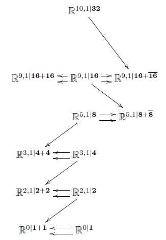
Hence the progression

of maximal invariant extensions of the superpoint

continues as a diagram

of super L-∞ algebras like so:

$\,$

$\,$

(While every extension displayed is a maximal invariant higher central extension, not all invariant higher central extensions are displayed. For instance there are string and membrane GS-WZW-terms / cocycles also on the lower dimensional super-Minkowski spacetimes (“non-critical”), e.g. the super 1-brane in 3d and the super 2-brane in 4d.)

$\,$

The “old brane scan” ran into a conundrum:

Given that superstrings and supermembranes

are nicely classified by super Lie algebra cohomology

why do the other super p-branes not show up similarly?

Where are the D-branes and the M5-brane?

$\,$

But now we see that we should look for

further higher cocycles

not on super Lie algebras

but on super L-∞ algebras.

$\,$

Proposition

(Chryssomalakos-Azcárraga-Izquierdo-Bueno 99, Sakaguchi 99, Fiorenza-Sati-Schreiber 13)

The higher WZW terms for the D-branes

are invariant super $L_\infty$-cocycles

on the higher extended super Minkowski spacetimes from above

$$\mu_{D p} \;\colon\; \mathfrak{string} \stackrel{\phantom{AAAAAAAA}}{\longrightarrow} B^{p+1}\mathbb{R} \,.$$

Similarly,

the higher WZW term for the M5-brane

is an invariant super $L_\infty$ 7-cocycle

of the form

$$\mu_{M5} \;\colon\; \mathfrak{m}2\mathfrak{brane} \stackrel{\phantom{AAAAAAAAA}}{\longrightarrow} B^6 \mathbb{R} \,.$$

$\,$

By the above, these cocycles classify

further higher super $L_\infty$-algebra extensions

$$\array{ \mathfrak{d}p\mathfrak{brane} \\ {}^{\mathllap{hofib(\mu_{D p})}}\downarrow \\ \mathfrak{string}_{IIA/B} &\underset{\mu_{D p}}{\longrightarrow}& B^{p+1}\mathbb{R} } \;\;\;\;\;\;\;\;\,\;\;\;\;\;\;\;\;\;\;\; \array{ \mathfrak{m}5\mathfrak{brane} \\ {}^{\mathllap{hofib(\mu_{M5})}}\downarrow \\ \mathfrak{m}2\mathfrak{brane} &\underset{\mu_{M5}}{\longrightarrow}& B^6 \mathbb{R} }$$

$\,$

Notice that all these are higher cocycles

except for that of the D0-brane, which is just a 2-cocycle.

The ordinary central extension that this classifies

is just that which grows the 11th M-theory dimension by the above example .

$$\array{ \mathbb{R}^{10,1\vert \mathbf{32}} \\ {}^{\mathllap{hofib(\mu_{D0})}} \downarrow \\ \mathbb{R}^{9,1\vert \mathbf{16} + \overline{\mathbf{16}}} &\underset{\mu_{D0} = i \, \overline{\psi} \Gamma_{11} \psi }{\longrightarrow}& B \mathbb{R} }$$

This may be thought of

as a super $L_\infty$-theoretic incarnation

of D0-brane condensation

(Polchinski 99, around p. 8).

$\,$

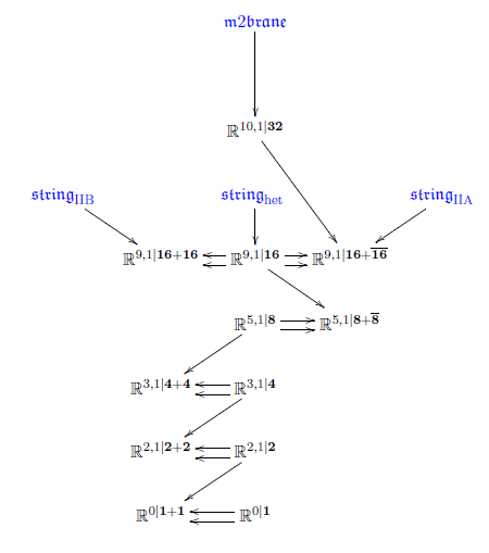
In conclusion:

by forming

iterated (maximal) invariant higher central super $L_\infty$-extensions

of the superpoint,

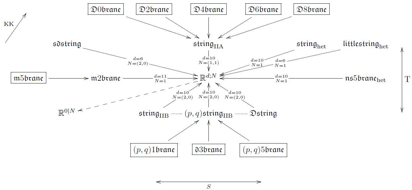
we obtain the following “brane bouquet”

$\,$

$\,$

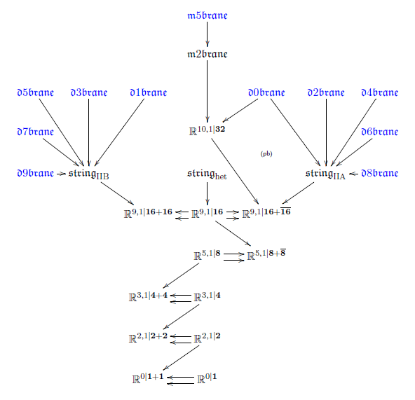
Each object in this diagram of super L-∞ algebras

is a super spacetime or super p-brane of string theory / M-theory.

$\,$

Moreover, this diagram knows the brane intersection laws:

there is a morphism $p_2\mathfrak{brane} \longrightarrow p_1 \mathfrak{brane}$

precisely if the given species of $p_1$-branes may end on the given species of $p_2$-branes

(more discussion of this is in Fiorenza-Sati-Schreiber 13, section 3).

$\,$

Perhaps we need to understand the nature of time itself better. $[...]$ One natural way to approach that question would be to understand in what sense time itself is an emergent concept, and one natural way to make sense of such a notion is to understand how pseudo-Riemannian geometry can emerge from more fundamental and abstract notions such as categories of branes. (G. Moore, p.41 of “Physical Mathematics and the Future”, talk at Strings 2014)

$\,$

But how are we to think of the extended super Minkowski spacetimes geometrically?

This is clarified by the following result:

$\,$

Proposition

(Fiorenza-Sati-Schreiber 13, section 5)

Write $\widetilde {String_{IIA}}$ for the super 2-group

that Lie integrates the super Lie 2-algebra $\mathfrak{string}_{IIA}$

subject to the condition that it carries a globally defined Maurer-Cartan form.

Then for $\Sigma_{p+1}$ a worldvolume smooth manifold

there is a natural equivalence

$$\left\{ \Sigma_{p+1} \stackrel{\Phi}{\longrightarrow} \widetilde{String_{IIA}} \right\} \;\;\; \leftrightarrow \;\;\; \left\{ \array{ \Sigma_{p+1} \stackrel{\phi}{\longrightarrow} \mathbb{R}^{9,1\vert \mathbf{16}+ \overline{\mathbf{16}} }, \\ \nabla \in Conn(\Sigma_{p+1}, \phi^\ast \mu_{string_{IIA}} ) } \right\}$$

between “higher Sigma-model fields” $\Phi$

and pairs, consisting of

an ordinary sigma-model field $\phi$

and a gauge field $\nabla$ on the worldvolume of the D-brane

twisted by the Kalb-Ramond field.

This is the Chan-Paton gauge field on the D-brane.

$\,$

Similarly:

Write $\widetilde {M2Brane}$ for the super 3-group

that Lie integrates the super Lie 3-algebra $\mathfrak{m}2\mathfrak{brane}$

subject to the condition that it carries a globally defined Maurer-Cartan form.

Then for $\Sigma_{5+1}$ a worldvolume smooth manifold

there is a natural equivalence

$$\left\{ \Sigma_{5+1} \stackrel{\Phi}{\longrightarrow} \widetilde{M2Brane} \right\} \;\;\; \leftrightarrow \;\;\; \left\{ \array{ \Sigma_{5+1} \stackrel{\phi}{\longrightarrow} \mathbb{R}^{10,1\vert \mathbf{32} }, \\ \nabla \in 2Conn(\Sigma_{p+1}, \phi^\ast \mu_{M2} ) } \right\}$$

between “higher Sigma-model fields” $\Phi$

and pairs, consisting of

an ordinary sigma-model field $\phi$

and a higher gauge field $\nabla$ on the worldvolume of the M5-brane

and twisted by the supergravity C-field.

$\,$

(See also at Structure Theory for Higher WZW Terms, session II).

$\,$

In conclusion this shows that

given a cocycle $\mu_{p_1+2}$ for some super $p_1$-brane species

inducing an extended super Minkowski spacetime via its homotopy fiber

and then given a consecutive cocycle $\mu_{p_2+2}$ for a $p_2$-brane species on that homotopy fiber

then $p_1$-branes may end on $p_2$-branes

and the $p_2$-branes propagating in the extended spacetime $p_1 \mathfrak{brane}$

see a higher gauge field on their worldvolume

of the kind sourced by boundaries of $p_1$-branes.

$\,$

$$\array{ { \text{spacetime} \atop \text{with}\,p_1\text{-brane condensate} } && p_1 \mathfrak{brane} &\overset{\mu_{p_2+2}}{\longrightarrow}& B^{p_2+2} \\ && {}^{\mathllap{hofib(\mu_{p_1+2})}}\downarrow \\ \text{spacetime} && \mathbb{R}^{d-1,1\vert \mathbf{N}} &\underset{\mu_{p_1+2}}{\longrightarrow}& B^{p_1+1}\mathbb{R} }$$

$\,$

Hence the extended super Minkowski spacetime $p_1 \mathfrak{brane}$

is like the original super spacetime $\mathbb{R}^{d-1,1\vert \mathbf{N}}$

but filled with a condensate of $p_1$-branes

whose boundaries source a higher gauge field.

$\,$

While this is good,

it means that at each stage of the brane bouquet

we are describing $p_2$-brane dynamics

on a fixed $p_1$-brane background field.

But more generally

we would like to describe the joint dynamics

of all brane species at once.

$\,$

This we turn to now.

$\,$

Fields

We now discuss that

$\;\;\;\;$There is homotopy descent of $p$-brane WZW terms

$\;\;\;\;$from extended super Minkowski spacetime

$\;\;\;\;$down to ordinary super Minkowski spacetime

$\;\;\;\;$which yields cocycles in twisted cohomology

$\;\;\;\;$for the RR-field and the M-flux fields.

(Fiorenza-Sati-Schreiber 15, 16a).

$\,$

In order to explain this we now first recall

the general nature of twisted cohomology

and its role in string theory.

$\,$

Twisted generalized cohomology

$\,$

It is often stated that a

Chan-Paton gauge field on $n$ coincident D-branes

is an SU(n)-vector bundle $V$,

hence a cocycle in nonabelian cohomology in degree 1.

$\,$

But this is not quite true.

In general there are $n$ D-branes and $n'$ anti-D-branes coinciding,

carrying Chan-Paton gauge fields

$V_{brane}$ (of rank $n$) and $V_{\text{anti-brane}}$ (of rank $n'$), respectively,

yielding a pair of vector bundles

$$(V_{\text{brane}}, V_{\text{anti-brane}}) \,.$$

Such pairs are also called virtual vector bundles.

$\,$

But D-branes annihilate with anti-D-branes (Sen 98)

when they have exact opposite D-brane charge,

which here means that they carry the same Chan-Paton vector bundle.

In other words, pairs as above of the special form

$(W,W)$ are equivalent to pairs of the form $(0,0)$.

$$(W,W) \;\sim\; 0 \,.$$

Hence the net Chan-Paton charge of coincident branes and anti-branes

is the equivalence class of $(V_{\text{brane}}, V_{\text{anti-brane}})$

under the equivalence relation which is generated by the relation

$$(V_{\text{brane}} \oplus W\,,\; V_{\text{anti-brane}} \oplus W) \;\sim\; (V_{brane}\,,\; V_{anti-brane})$$

for all complex vector bundles $W$ (Witten 98, Witten 00).

$\,$

The additive abelian group of such equivalence classes of virtual vector bundles

is called topological K-theory.

This behaves in many ways as ordinary cohomology does, but is richer.

One says that it is a generalized cohomology theory.

$\,$

It follows that also the RR-fields are in K-theory (Moore-Witten 00).

$\,$

Topological K-theory is similar to ordinary cohomology

but is a generalized (Eilenberg-Steenrod) cohomology theory.

A generalized cohomology theory is represented by a spectrum

(in the sense of stable homotopy theory):

A spectrum is a sequence of pointed topological spaces

$$E_n \;\;\;\; n \in \mathbb{N}$$

equipped with weak homotopy equivalences

$$E_n \overset{\phantom{AA}\simeq\phantom{AA}}{\longrightarrow} \Omega E_{n+1}$$

from one to the loop space of the next.

$\$

Given this, then the $E$-cohomology of any topological space $X$ is

$$E^n(X) \coloneqq \underset{\text{homotopy classes of maps}}{\underbrace{\pi_0\left\{ X \overset{\phantom{AAAAAA}}{\longrightarrow} E_n \right\} }} \,.$$

For topological K-theory one writes

$$E = KU$$

with

$$KU_{2n} \simeq B U \times \mathbb{Z} \;\;\,,\;\; KU_{2n+1} \simeq U$$

with $U$ the stable unitary group,

and $B U$ the classifying space for complex vector bundles.

$\,$

But above we saw

that the Chan-Paton gauge field on a D-brane

is actually a twisted vector bundle

with twist given by the Kalb-Ramond field

sourced by a string condensate.

(Freed-Witten anomaly cancellation)

$\,$

Such twisted cohomology generalized cohomology is given by

1. a classifying space of twists $B G$

2. a spectrum object in the slice category $Top_{/B G}$, namely a sequence of spaces $E_n/G$ equipped with maps

   $$id \;\colon\; B G \to E_n/G \to B G$$

   and weak equivalences

   $$E_n/G \overset{\phantom{AA}\simeq\phantom{AA} }{\longrightarrow} \Omega_{B G} (E_{n+1}/G) \coloneqq \underset{\text{homotopy} \atop {\text{fiber} \atop \text{product} } }{\underbrace{ B G \underoverset{E_{n+1}/G}{h}{\times} B G }}$$

Extremal examples:

1. an ordinary spectrum $E$

   is a parameterized spectrum over the point;

   $$\array{ E \\ \downarrow \\ \ast }$$

2. an ordinary space $X$

   is identified with the zero-spectrum parameterized over $X$:

   $$\array{ X \\ \downarrow^{\mathrlap{id}} \\ X }$$

Then

1. a twist $\tau$ for $E$-cohomology of $X$ is a map

   $$\array{ X \\ & {}_{\mathllap{\tau}}\searrow \\ && B G }$$

2. the $\tau$-twisted $E$-cohomology of $X$ is

   $$E^{n+\tau}(X) \;\coloneqq\; \pi_0 \left\{ \array{ X && \longrightarrow && E_n/G \\ & {}_{\mathllap{\tau}} \searrow && \swarrow_{\mathrlap{}} \\ && B G } \right\}$$

There is a homotopy fiber sequence (in parameterized spectra)

$$\array{ E &\longrightarrow& E/G \\ && \downarrow \\ && B G }$$

and this equivalently exhibits $E/G$ as the homotopy quotient of an ordinary spectrum $E$ by a $G$-infinity-action.

(Nikolaus-Schreiber-Stevenson 12, section 4.1)

$\,$

Assume that $B G$ is simply connected, i.e. of the form $B^2 G$.

$\,$

We now translate this situation to super L-∞ algebras

via the central theorem of rational homotopy theory.

$\,$

Rational homotopy theory

$\,$

On every loop space $\Omega X$,

the operation of concatenation of loops

gives the structure of a group up to coherent higher homotopy

called a “grouplike A-∞ space”

or ∞-group for short.

$\,$

May recognition theorem:

Conversely, for $G$ an ∞-group

there is an essentially unique connected space $B G$

with $G \;\simeq\; \Omega B G$.

$\,$

Every double loop space $\Omega \Omega X$

becomes a “first order abelian” ∞-group

by exchanging loop directons

called a braided ∞-group,

$\,$

For $G$ a braided ∞-group then

$B G$ is itself an ∞-group

and so there exists an essentially unique simply connected space

$$B^2 G \coloneqq B (B G)$$

with

$$G \;\simeq\; \Omega^2 B^2 G \,.$$

$\,$

And so forth:

Every triple loop space $\Omega^3 X$

becomes a “second order abelian” ∞-group

by exchanging loop directons

called a sylleptic ∞-group.

etc.

$\,$

In a spectrum $E$,

the maps $E_n \stackrel{\simeq}{\to} \Omega E_{n+1}$

exhbit $E_0$ as an infinite loop space

hence as a fully abelian ∞-group.

$\,$

It turns out that by a homotopy theoretic version of Lie theory,

there is an L-∞ algebra $\mathfrak{g}$ associated with any ∞-group

$$\mathfrak{g} \simeq \mathfrak{l} B G \,.$$

or

$$B\mathfrak{g} \simeq \mathfrak{l} B^2 G$$

etc.

$\,$

Its Chevalley-Eilenberg algebra $CE(\mathfrak{B g})$

is called a Sullivan model for $B^2 G$.

$\,$

For example the $L_\infty$-algebra associated with an Eilenberg-MacLane space

$$K(\mathbb{Z},n+1) \simeq B^{n+1}\mathbb{Z}$$

is the line Lie-n algebra from above:

$$\mathfrak{l}(B^{n+1} \mathbb{Z}) \;\simeq\; B^n \mathbb{R} \,.$$

$\,$

The main theorem of rational homotopy theory (Quillen 69, Sullivan 77)

says that the L-∞ algebra $\mathfrak{l}(B^2 G)$ equivalently reflects the rationalization of $B^2 G$

(in fact the real-ification, since we are considering $L_\infty$-algebras over the real numbers).

This means that weak equivalence between $L_\infty$-algebras correspond to maps between spaces

that induce isomorphism on real-ified homotopy groups

$$\left\{ \;\;\;\;\; \array{ B^2 G_1 \overset{\phantom{AA}f\phantom{AA}}{\longrightarrow} B^2 G_2 \\ \text{such that:} \\ \pi_\bullet(B^2 G_1)\otimes_{\mathbb{Z}} \mathbb{R} \underoverset{\simeq}{\pi_\bullet(f) \otimes_{\mathbb{Z}} \mathbb{R} }{\longrightarrow} \pi_\bullet(B^2 G_2) \otimes_{\mathbb{Z}} \mathbb{R} } \;\;\;\;\; \right\} \;\;\;\leftrightarrow\;\;\; \left\{ \; \mathfrak{l}(B^2 G_1) \stackrel{\simeq}{\longrightarrow} \mathfrak{l}(B^2 G_2) \; \right\} \,.$$

For concise review in the language that we use here see Buijs-Félix-Murillo 12, section 2.

$\,$

We apply this rational homotopy theory functor

$$\mathfrak{l}(-) \;\colon\; \text{Spaces} \longrightarrow L_\infty\text{-Algebras}$$

to find the $L_\infty$-algebraic version of parameterized spectra

hence of twisted cohomology:

$\,$

$$\array{ { \text{parameterized} \atop \text{spectrum} } \;\;\;&\;\;\;\; \left\{ \array{ id : B^2 G \to E_n/ B G \to B^2 G \\ E_n/ B G \stackrel{\simeq}{\longrightarrow} \Omega_{B^2 G} (E_{n+1}/ B G) } \right\} \;&\;\leftrightarrow\;&\; \left( \array{ E &\longrightarrow& E/B G \\ && \downarrow \\ && B^2 G } \right) \\ & \mathfrak{l}(-)\downarrow \\ L_\infty\text{Algebra} \;\;\;&\;\;\;\; \left\{ \array{ id : \mathfrak{l}(B^2 G) \to \mathfrak{l}(E_n/ B G) \to \mathfrak{l}(B^2 G) \\ \mathfrak{l}(E_n/ B G) \stackrel{\simeq}{\longrightarrow} \Omega_{\mathfrak{l}(B^2 G)} \mathfrak{l}(E_{n+1}/ B G) } \right\} \;&\;\leftrightarrow\;&\; \left( \array{ V[1] &\longrightarrow& V[1]/\mathfrak{g} \\ && \downarrow \\ && B \mathfrak{g} } \right) }$$

$\,$

Here $V \simeq E \otimes \mathbb{R}$ is a chain complex

underlying the real-ification of the spectrum $E$

(stable Dold-Kan correspondence).

$\,$

So for $\mathbb{R}^{d-1,1\vert \mathbf{N}}$ some super Minkowski spacetime, a cocycle in $\mathfrak{g}$-twisted $V$-cohomology is a diagram of the form

$$\array{ \mathbb{R}^{d-1,1\vert \mathbf{N}} && \overset{}{\longrightarrow} && V/\mathfrak{g} \\ & \searrow && \swarrow \\ && B \mathfrak{g} }$$

$\,$

Now given one stage in the brane bouquet

$$\array{ \widehat{\widehat{\mathfrak{g}}} \\ {}^{\mathllap{hofib(\mu_{p_2})}}\downarrow \\ \hat \mathfrak{g} & \stackrel{\mu_{p_2}}{\longrightarrow} & B\mathfrak{h}_2 \\ {}^{\mathllap{hofib(\mu_{p_1})}}\downarrow \\ \mathfrak{g} &\overset{\mu_{p_1}}{\longrightarrow}& B\mathfrak{h}_1 }$$

we want to descent $\mu_{p_2}$ to $\mathfrak{g}$.

$\,$

By the general theory of principal ∞-bundles (Nikolaus-Schreiber-Stevenson 12):

1. $\widehat{\mathfrak{g}}$ has a $\mathfrak{h}_1$-∞-action

2. equipping $B \mathfrak{h}_2$ with an $\mathfrak{h}_1$-∞-action

   is equivalent to finding a homotopy fiber sequence as on the right here:

   $$\array{ \hat \mathfrak{g} && \stackrel{\mu_2}{\longrightarrow} && \mathbf{B}\mathfrak{h}_2 \\ {}^{\mathllap{hofib(\mu_1)}}\downarrow && && \downarrow^{\mathrlap{hofib(p_\rho)}} \\ \mathfrak{g} && && (\mathbf{B}\mathfrak{h}_2)/\mathfrak{h}_1 \\ & {}_{\mathllap{\mu_1}}\searrow && \swarrow_{\mathrlap{p_\rho}} \\ && \mathbf{B}\mathfrak{h}_1 } \,.$$

3. $\mu_2$ is $\mathfrak{h}_1$-equivariant precisely if it descends to a morphism

   $$\mu_2/\mathfrak{h}_1 \;\colon\; \mathfrak{g} \longrightarrow (\mathbf{B}\mathfrak{h}_2)/\mathfrak{h}_1$$

   such that this diagram commute up to homotopy:

   $$\array{ \hat \mathfrak{g} && \stackrel{\mu_2}{\longrightarrow} && \mathbf{B}\mathfrak{h}_2 \\ {}^{\mathllap{hofib(\mu_1)}}\downarrow && && \downarrow^{\mathrlap{hofib(p_\rho)}} \\ \mathfrak{g} && \stackrel{\mu_2/\mathfrak{h}_1}{\longrightarrow} && (\mathbf{B}\mathfrak{h}_2)/\mathfrak{h}_1 \\ & {}_{\mathllap{\mu_1}}\searrow && \swarrow_{\mathrlap{p_\rho}} \\ && \mathbf{B}\mathfrak{h}_1 } \,.$$

4. if so, then resulting triangle diagram

   $$\array{ \mathfrak{g} && \stackrel{\mu_2/\mathfrak{h}_1}{\longrightarrow} && (\mathbf{B}\mathfrak{h}_2)/\mathfrak{h}_1 \\ & {}_{\mathllap{\mu_1}}\searrow && \swarrow_{\mathrlap{p_\rho}} \\ && \mathbf{B}\mathfrak{h}_1 }$$

   exhibits $\mu_2/\mathfrak{h}_1$ as a cocycle in (rational) $\mu_1$-twisted cohomology

   with respect to the local coefficient bundle $p_\rho$.

$\,$

We now work out this general prescription

for the cocycles in the brane bouquet.

$\,$

RR-fields

$\,$

By the brane bouquet above

the type IIA D-branes

are given by super $L_\infty$ cocycles of the form

$$\mathfrak{string}_{IIA } \overset{\mu_{Dp}}{\longrightarrow} B^{p+1}\mathbb{R}$$

for $p \in \{0,2,4,6,8,10\}$.

$\,$

Notice that

$$H^\bullet(B U, \mathbb{Z})$$

has one generator in each even degree, the universal Chern classes.

Hence the $L_\infty$-algebra

$$\mathfrak{l}(KU)$$

is given by

$$CE(\mathfrak{l}(KU)) \;\simeq\; \left\{ d \omega_{2p+2} = 0 \;\vert\; p \in \mathbb{Z} \right\} \,.$$

This allows to unify the D-brane cocycles

into a single morphism of super $L_\infty$-algebras of the form

$$\array{ \mathfrak{string}_{IIA} && \stackrel{\phantom{AA}\mu_D\phantom{AA}}{\longrightarrow} && \mathfrak{l}(KU) \\ {}^{\mathllap{hofib(\mu_{F1})}}\downarrow \\ \mathbb{R}^{9,1\vert \mathbf{16}+ \overline{\mathbf{16}}} \\ & {}_{\mathllap{\mu_{F1}}}\searrow \\ && \mathbf{B}^2 \mathbb{R} } \,.$$

$\,$

By the above prescription, descending $\mu_D$ is equivalent

to finding a commuting diagram in the homotopy category of super $L_\infty$-algebras

of the form

$$\array{ \mathfrak{string}_{IIA} && \stackrel{\phantom{AA}\mu_D\phantom{AA}}{\longrightarrow} && \mathfrak{l}(KU) \\ {}^{\mathllap{hofib(\mu_{F1})}}\downarrow && && \downarrow^{\mathrlap{hofib(\phi)}} \\ \mathbb{R}^{9,1\vert \mathbf{16}+ \overline{\mathbf{16}}} &&\overset{\phantom{AA}\mu_{D}/B \mathbb{R}\phantom{AA} }{\longrightarrow}&& \text{something} \\ & {}_{\mathllap{\mu_{F1}}}\searrow && \swarrow_{\mathrlap{\phi}} \\ && \mathbf{B}^2 \mathbb{R} } \,.$$

$\,$

This turns out to exist as follows (Fiorenza-Sati-Schreiber 16a, section 5):

Define the $L_\infty$-algebra

$$\mathfrak{l}(KU / BU(1))$$

by

$$CE\left(\mathfrak{l}(KU / BU(1))\right) \;=\; \left\{ \array{ d h_3 = 0\;,\; \\ d \omega_{2p+2} = h_3 \wedge \omega_{2p} } \right\} \,.$$

Moreover write

$$\mathbb{R}^{9,1\vert \mathbf{16} + \overline{\mathbf{16}}}_{res}$$

for the super $L_\infty$-algebra whose Chevalley-Eilenberg algebra is

$$CE\left( \mathbb{R}^{9,1\vert \mathbf{16} + \overline{\mathbf{16}}}_{res} \right)[f_2,h_3]/(d f_2 = \mu_{F1} + h_3)$$

$\,$

Proposition

(Fiorenza-Sati-Schreiber 16a, theorem 4.16)

The super $L_\infty$-algebra $\mathbb{R}^{9,1\vert \mathbf{16} + \overline{\mathbf{16}}}_{res}$

is a resolution of type IIA super-Minkowski spacetime.

in that there is a weak equivalence

$$\mathbb{R}^{9,1\vert \mathbf{16} + \overline{\mathbf{16}}}_{res} \stackrel{\phantom{AA}\simeq\phantom{AA}}{\longrightarrow} \mathbb{R}^{9,1\vert \mathbf{16} + \overline{\mathbf{16}}} \,.$$

This fits into a commuting diagram of the form

$$\array{ \left\{ {{d e^a = \overline{\psi}\Gamma^a \wedge \psi } \atop {d \psi^\alpha = 0}} \atop { d f_2 = \mu_{F1}} \right\} && \mathfrak{string}_{IIA} && \stackrel{ \mu_D }{\longrightarrow} && \mathfrak{l}(KU) && \left\{ d \omega_{2 p+2} = 0 \right\} \\ && \downarrow^{\mathrlap{hofib(\mu_{F1})}} && && \downarrow^{\mathrlap{\phi}} \\ \left\{ {{d e^a = \overline{\psi}\Gamma^a \wedge \psi } \atop {d \psi^\alpha = 0}} \atop { d f_2 = \mu_{F1} + h_3 } \right\} & & \mathbb{R}_{res}^{9,1\vert \mathbf{16}+ \overline{\mathbf{16}}} && \stackrel{ \mu_{F1/D} }{\longrightarrow} && \mathfrak{l}(KU / B U(1)) && \left\{ d\omega_{2p+2} = h_3\wedge \omega_{2p} \right\} \\ && & {}_{\mathllap{\mu_{F 1}}}\searrow && \swarrow_{\mathrlap{\phi}} \\ && && \mathbf{B}^2 \mathbb{R} \\ && && \left\{ d h_3 = 0 \right\} } \,.$$

$\,$

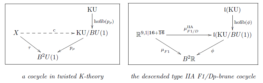
In conclusion

$\;\;$the type IIA F1-brane and D-brane cocycles with $\mathbb{R}$-coefficients

$\;\;$do descent to super-Minkowski spacetime

$\;\;$as one single cocycle with coefficients

$\;\;$in rationalized twisted K-theory.

$\,$

M-flux fields

$\,$

The part of the brane bouquet giving the M-branes is

$$\array{ \mathfrak{m}2\mathfrak{brane} &\stackrel{\mu_{M5}}{\longrightarrow}& \mathbf{B}^6 \mathbb{R} \\ {}^{\mathllap{hofib(\mu_{M2})}}\downarrow \\ \mathbb{R}^{10,1\vert \mathbf{32}} & \stackrel{\mu_{M2}}{\longrightarrow} & \mathbf{B}^3 \mathbb{R} \\ {}^{\mathllap{hofib(\mu_{D 0})}}\downarrow \\ \mathbb{R}^{9,1\vert \mathbf{16} + \overline{\mathbf{16}}} }$$

$\,$

In order to descend this, consider the $L_\infty$-algebra corresponding to the 4-sphere

$$\mathfrak{l}(S^4) \,.$$

By standard results on rational n-spheres, this is given by

$$CE(\mathfrak{l}S^4) \;\simeq\; \left\{ \array{ d \, g_4 = 0\,,\, \\ d\, g_7 + \tfrac{1}{2} g_4 \wedge _4 = 0 } \right\} \,.$$

Proposition

Fiorenza-Sati-Schreiber 15, section 3

There is a homotopy fiber sequence of $L_\infty$-algebras as on the right

$$\left( \array{ && S^7 \\ && \downarrow \\ && S^4 \\ & \swarrow \\ B SU(2) \\ \downarrow^{\mathrlap{c_2}} \\ B^3 U(1) } \right) \;\; \stackrel{\phantom{AA}\mathfrak{l}(-)\phantom{AA} }{\mapsto} \;\; \left( \array{ && B^6 \mathbb{R} \\ && \downarrow^{\mathrlap{ hofib(\mathfrak{l}(c_2)) } } \\ &&\mathfrak{l}(S^4) \\ & \swarrow_{\mathfrak{l}(c_2)} \\ B^3 \mathbb{R} } \;\;\;\;\;\;\;\;\;\;\;\;\;\;\;\; \right)$$

which is the image under $\mathfrak{l}(-)$ of the quaternionic Hopf fibration.

This makes a commuting diagram

in the homotopy category of super $L_\infty$-algebas

of the form

$$\array{ \left\{ { { d e^a = \overline{\psi}\wedge \Gamma^a \wedge \psi } \atop { d \psi^\alpha = 0 } } \atop d h_3 = - \mu_{M2} \right\} && \mathfrak{m}2\mathfrak{brane} && \stackrel{ \mu_{M5} }{\longrightarrow} && B^6 \mathbb{R} && \left\{ d g_7 = 0 \right\} \\ && \downarrow^{\mathrlap{hofib(\mu_{M2})}} && && \downarrow^{\mathrlap{hofib(\mathfrak{l}(c_2))}} \\ \left\{ { { d e^a = \overline{\psi}\wedge \Gamma^a \wedge \psi } \atop { d \psi^\alpha = 0 } } \atop d h_3 = g_4 - \mu_{M2} \right\} && \mathbb{R}_{res}^{10,1\vert\mathbf{32}} && \stackrel{ \mu_{M2/M5} }{\longrightarrow} && \mathfrak{l} S^4 && \left\{ {d g_4 = 0} \atop {d g_7 + \tfrac{1}{2} g_4 \wedge g_4 = 0} \right\} \\ && & {}_{\mathllap{\mu_{M2}}}\searrow && \swarrow_{\mathrlap{\mathfrak{l}(c_2)}} \\ && && \mathbf{B}^3 \mathbb{R} \\ && && \left\{ d g_4 = 0\right\} }$$

In conclusion

$\;\;$this says that, rationally,

$\;\;$M2-brane charge is in degree-4 ordinary cohomology

$\;\;$and it twists M5-brane charge

$\;\;$which is, rationally, in unstable degree-4 cohomotopy.

$\,$

This confirms a conjecture due to

(Sati 10, section 6.3, Sati 13, section 2.5).

based on the observation that

the equations of motion of 11-dimensional supergravity

for the supergravity C-field field strength $G_4$ say that

$$d G_7 + \tfrac{1}{2} G_4 \wedge G_4 = 0$$

with $G_7 = \ast G_4$ the Hodge dual

and this is just the algebraic relation for the Sullivan model of the rational 4-sphere.

$\,$

Notice that, unstably, the 4-sphere

is just the space whose non-torsion homotopy groups

hence those that are visible in rational homotopy theory

are in degrees 2+2 and 5+2:

k	1	2	3	4	5	6	7
$\phantom{AA}\pi_k(S^4)\phantom{AA}$	$\phantom{AA}0\phantom{AA}$	$\phantom{AA}0\phantom{AA}$	$\phantom{AA}0\phantom{AA}$	$\phantom{AA}\mathbb{Z}\phantom{AA}$	$\phantom{AA}\mathbb{Z}/2\phantom{AA}$	$\phantom{AA}\mathbb{Z}/2\phantom{AA}$	$\phantom{AA}\mathbb{Z} \oplus \mathbb{Z}/{12}\phantom{AA}$

$\,$

But the correct non-rational lift of the $\mathfrak{l}(S^4)$-coefficients

will also have to be such that it somehow gives rise to twisted K-theory

under double dimensional reduction. This is still an open problem.

For further comments see the talk

Equivariant cohomology of M2/M5-branes

$\,$

$\,$

Now that we have found

the descended $L_\infty$-cocycles

for all super $p$-branes

in twisted cohomology, rationally,

we may analyze their behaviour under double dimensional reduction

and discover the super $L_\infty$-algebraic incarnation

of various dualities in string theory.

$\,$

$\,$

Double dimensional reduction

$\,$

Underlying most of the dualities in string theory is

the phenomenon of double dimensional reduction

so called because:

1. the dimension of spacetimes is reduced

   by Kaluza-Klein compactification on a fiber $F$;

2. in parallel the dimension of branes is reduced

   if they wrap $F$.

$\,$

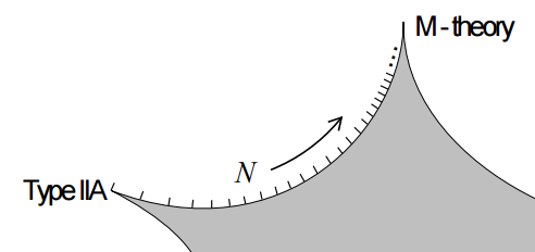
For example double dimensional reduction is supposed to underly

the duality between M-theory and type IIA string theory:

• spacetime$X_{11}$ is an 11d circle-fiber bundle

  locally of the form $X_{11} = X_{10} \times S^1$

  over a 10d base spacetime;

• an M-theory membrane (M2-brane) with cyclindrical worldvolume

  $$\Sigma_3 = \Sigma_2 \times S^1$$

  wraps the circle fiber if its trajectory

  $$\phi_{M2} \;\colon\; \Sigma_3 \longrightarrow X_{11}$$

  is of the form

  $$\phi_{F1} \times \mathrm{id}_{S^1} \;\colon\; \Sigma_2 \times S^1 \longrightarrow X_{10} \times S^1 \,.$$

As the Riemannian circumference of the circle fiber $S^1$ tends towards zero

this effectively looks like the 2-dimensional worldsheet $\Sigma_2$ of a string

tracing out a trajectory in 10-dimensional spacetime:

$$\phi_{F1} \;\colon\; \Sigma_2 \longrightarrow X_{10}$$

$\,$

But there is also “single dimensional reduction”

when the membrane does not wrap the fiber space:

$$\array{ \Sigma_3 && \overset{\phi_{M2}}{\longrightarrow} && X_{11} \\ & {}_{\phi_{D2}}\searrow && \nearrow \\ && X_{10} }$$

In this case it looks like a membrane in 10d spacetime,

now called the D2-brane.

$\,$

Similarly the M5-brane in M-theory

$$\phi_{M5} \;\colon\; \Sigma_{6} \longrightarrow X_{11}$$

may wrap the circle fiber

to yield a 4-brane in 10d, called the D4-brane

or it may not wrap the circle fiber

to yield a 5-brane in 10d, called the NS5-brane.

$\,$

Beware the naive treatment of branes in this traditional argument.

And even naively, this is not the full story yet:

The $S^1$-fibration itself is supposed to re-incarnate in 10d

as the D0-brane and the D6-brane.

$\,$

Hence double dimensional reduction from M-theory to type IIA string theory

is meant to, schematically, involve decompositions as follows

$$\underset{spacetime}{ \underbrace{ \array{ X_{11} \\ \downarrow^{\pi} \\ X_{10} } } } \;\; \underset{branes}{ \underbrace{ \array{ && && \text{M2-brane} && && && \text{M5-brane} \\ && & {}^{\mathllap{wrapped}}\swarrow && \searrow^{\mathrlap{not \atop wrapped}} & & && {}^{\mathllap{wrapped}}\swarrow && \searrow^{\mathrlap{not \atop wrapped}} \\ \text{D0-brane} && \text{F1-brane} && && \text{D2-brane} && \text{D4-brane} && && \text{NS5-brane} } } }$$

$\,$

Above we saw that all super p-branes are

characterized by the flux fields $H_{p+2}$ that they are charged under,

more precisely by the bispinorial component of $H_{p+2}$

which is constrained to be super-tangent-space-wise the form

$$H_{p+2}^{fermionic} \;=\; \tfrac{i^{p(p-1)/2}}{p!} \, \left( \overline{\Psi} \wedge \Gamma_{a_1 \cdots a_p}\Psi \right) \wedge E^{a_1} \wedge \cdots \wedge E^{a_p}$$

where $(E^a, \Psi^\alpha)$ is the super vielbein (graviton and gravitino).

$\,$

$\,$

Hence we will formalize double dimensional reduction in terms of these fields.

$\,$

Again there is a naive picture to help the intuition:

Let $G_4 \in \Omega^4_{cl}(X_{11})$ be the differential 4-form flux field strength of the supergravity C-field.

Under the Gysin sequence for the spherical fibration

$$\array{ S^1 &\hookrightarrow& X_{11} \\ && \downarrow^{\mathrlap{\pi}} \\ && X_{10} }$$

this decomposes in cohomology as

$$G_4 = (d x^{10}) \wedge H_3 + \pi^\ast F_4$$

thus giving rise in 10d to

1. a 3-form $H_3$, the Kalb-Ramond B-field field strength that the string couples to;

2. a 4-form $F_4$, the RR-field field strength in degree 4, that the D2-brane couples to.

Similary the 7-form field strength $G_7$ decomposes as

$$G_7 = (d x^{10}) \wedge F_6 + \pi^\ast H_7$$

thus giving rise in 10d to

1. a 6-form $F_6$, the RR-field field strength in degree 6, that the D4-brane couples to

2. a 7-form $H_7$, the dual NS-NS field strength that the NS5-brane couples to.

$$\underset{spacetime}{ \underbrace{ \array{ X_{11} \\ \downarrow^{\pi} \\ X_{10} } } } \;\; \underset{fluxes}{ \underbrace{ \array{ && && G_4\text{-flux} && && && G_7\text{-flux} \\ && & {}^{\mathllap{wrapped}}\swarrow && \searrow^{\mathrlap{not \atop wrapped}} & & && {}^{\mathllap{wrapped}}\swarrow && \searrow^{\mathrlap{not \atop wrapped}} \\ F_2\text{-flux} && H_3\text{-flux} && && F_4\text{-flux} && F_6\text{-flux} && && H_7\text{-flux} } } }$$

$\,$

The advantage of this perspective on double dimensional reduction

from the point of view of the background flux fields

is that powerful tools from cohomology theory apply.

$\,$

To first approximation

background fluxes represent classes in ordinary cohomology (their charges).

There is a classifying space $B^n \mathbb{Z}$ for ordinary cohomology

$$H^n(X,\mathbb{Z}) \;\;\; \simeq \;\;\; \left\{ \array{ \text{continuous functions} \\ X \longrightarrow B^n \mathbb{Z} } \right\}_{/homotopy}$$

(called an Eilenberg-MacLane space, often denoted $K(\mathbb{Z},n)$).

Hence the charge of $G_4$/$G_7$-flux, to first approximation, is represented by a classifying map

$$([G_4], [G_7]) \;\colon\; X_{11} \longrightarrow B^4 \mathbb{Z} \,\times\, B^7 \mathbb{Z} \,.$$

and we saw that under double dimensional reduction

this is supposed to transmute into a map of the form

$$([F_2] , [H_3], [F_4], [F_6], [H_7]) \;\colon\; X_{10} \longrightarrow B^2 \mathbb{Z} \;\times\; B^3 \mathbb{Z} \;\times\; B^4 \mathbb{Z} \;\times\; B^6 \mathbb{Z} \;\times\; B^7 \mathbb{Z} \,.$$

$\,$

Which mathematical operation could cause such a transmutation?

We will now find such an operation

and then use it to give an improved definition of double dimensional reduction,

one that knows about all the fine print of brane charges.

$\,$

Via free looping (no 0-brane effect)

$\,$

Let’s first record formally

what was going on in the above story.

$\,$

In the above double dimensional reduction

of the naive M-fluxes on a trivial 11d circle bundle

we used

1. the Cartesian product with the circle

2. functions out of the circle.

Let’s have a closer look at these two operations:

$\,$

It is a classical fact about locally compact topological spaces

(which includes all topological spaces that one cares about in physics)

that

given topological spaces $\Sigma$, $X$ and $F$, then there is a natural bijection

$$\left\{ \array{ \text{continuous functions} \\ \Sigma \times F \longrightarrow X } \right\} \;\; \underoverset {\text{"forming adjuncts"}} {\simeq} {\leftrightarrow} \;\; \left\{ \array{ \text{continous functions} \\ \Sigma \longrightarrow Maps(F,X) } \right\}$$

where

• $F \times X$ is the product topological space of $F$ with $X$

  (the set of pairs of points euipped with the product topology)

• $Maps(F,Y)$ is the mapping space from $F$ to $X$,

  (the set of continuous functions) $F \to X$ equipped with the compact-open topology)

Except for the subtlety with the topology

this bijection is just rewriting

a function of two variables as a function with values in a second function

$$(\tilde f(a))(b) = f(a,b) \,.$$

$\,$

One says that the two functors

$$Top_{cg} \; \underoverset {\underset{Maps(F,-)}{\longrightarrow}} {\overset{F \times (-)}{\longleftarrow}} {\bot} \; Top_{cg}$$

form a adjoint pair or an adjunction.

$\,$

$\,$

A remarkable amount of structure comes with every adjunction:

• the adjunct of the identity $F \times X \overset{id}{\to} F \times X$

  generally called the unit of the adjunction,

  here is the wrapping operation

  $$X \overset{}{\longrightarrow} Maps(F, F \times X)$$

• the adjunct of the identity $Maps(F,X) \overset{id}{\to} Maps(F,X)$

  generally called the counit of the adjunction,

  here is the evaluation map

  $$F \times Maps(F, X) \overset{ev}{\longrightarrow} X$$

  that evaluates a function on an argument

$\,$

We will see now that the following general fact

about adjoint functors

serves to implement the above physics story

of wrapped branes:

$\,$

Fact.

The adjunct of a map of the form

$$G \;\colon\; F \times X \overset{}{\longrightarrow} A$$

is the composite of its image under $Maps(F,-)$ with the adjunction unit $\eta_X$:

$$\tilde G \;\colon\; X \overset{\eta_X}{\longrightarrow} Maps(F,F \times X) \overset{Maps(F,G)}{\longrightarrow} Maps(F,A)$$

$\,$

Moreover, we will see that the following generall fact in homotopy theory

accurately implements the idea of dimensional reduction of the brane dimensions:

$\,$

For $F = S^1$ the circle, then

$$\mathcal{L} X \;\coloneqq\; Maps(S^1, X)$$

is also called the free loop space of $X$.

$\,$

Proposition

For $G$ a general topological group, then its free loop space

$$Maps(S^1, B G) \;\simeq\; G/_{ad}G$$

is weakly homotopy equivalent to the

homotopy quotient of $G$ by its adjoint action.

In the special case that $G$ is an abelian topological group.

then this becomes a weak homotopy equivalence of following simple form

$$Maps(S^1 , B G) \; \simeq \; \underset{\text{wrapped} \atop \text{coefficient}}{\underbrace{G}} \; \times \; \underset{\text{plain} \atop \text{coefficient} }{\underbrace{ B G }} \,.$$

This captures the required reduction on brane dimension!

$\,$

In particular if $G = B^n \mathbb{Z}$ then

$$Maps(S^1, B^{n+1} \mathbb{Z}) \;\; \simeq B^n \mathbb{Z} \;\times\; B^{n+1} \mathbb{Z} \,.$$

$\,$

$\,$

Example

Consider naive $M$-flux fields $G_4$ and $G_7$

on an 11d spacetime that is a trivial circle bundle $X_{11} = X_{10} \times S^1$.

Its charges is represented by a map of the form

$$([G_4], [G_7]) \;\colon\; X_{10} \times S^1 \longrightarrow B^4 \mathbb{Z} \times B^7 \mathbb{Z} \,.$$

By adjunction this is identified with a map of the form

$$\left([H_3], [F_4], [F_6], [H_7]\right) \,\coloneqq\, \widetilde{([G_4], [G_7])} \;\colon\; X_{10} \longrightarrow Maps\left( S^1, \; B^4 \mathbb{Z} \times B^7 \mathbb{Z} \; \right) \;\;\simeq\;\; B^3 \mathbb{Z} \;\times\; B^4 \mathbb{Z} \;\times\; B^6 \mathbb{Z} \;\times\; B^7 \mathbb{Z} \,.$$

where on the right we have the transmuted coefficients by prop.

This is exactly the result we were after.

$\,$

Better yet, the adjunction yoga

accurately reflects the physics story:

For consider a $p$-brane propagating in 10d spacetimes along a trajectory

$$\phi_p \;\colon\; \Sigma_p \longrightarrow X_{10}$$

and coupled to these dimensionally reduced background fields

$$\Sigma_p \overset{\phi_p}{\longrightarrow} X_{10} \overset{([H_3], [F_4], [F_6], [H_7])}{\longrightarrow} B^3 \mathbb{Z} \;\times\; B^4 \mathbb{Z} \;\times\; B^6 \mathbb{Z} \;\times\; B^7 \mathbb{Z} \;\;\;\simeq\;\;\; Maps(S^1, B^4 \mathbb{Z} \,\times\, B^7 \mathbb{Z}) \,.$$

By adjunction this is identified with a map of the form

$$\Sigma_p \times S^1 \overset{\phi_p \times S^1}{\longrightarrow} X_{10} \times S^1 = X_{11} \overset{([G_4], [G_7])}{\longrightarrow} B^4 \mathbb{Z} \;\times\; B^7 \mathbb{Z}$$

and this is exactly the coupling we saw in the story of double dimensional reduction.

$\,$

So this works well as far as it goes, but

so far it only applies to trivial circle fibrations

and it does not see the D0-charge.

$\,$

We now disucss the improvement to the full formulation.

$\,$

$\,$

Via cyclification (with 0-brane effects)

In general the M-theory circle bundle

$$\array{ S^1 &\hookrightarrow& X_{11} \\ && \downarrow \\ && X_{10} }$$

is only locally a product with of $X_{10}$ with $S^1$.

$\,$

For example

the complement of the locus of a KK-monopole spacetime

is a circle principal bundle with first Chern class

equal to the charge carried by the KK-monopole.

(which is the corresponding number of coincident D6-branes in type IIA).

$\,$

Hence in general the above formulation of double dimensional reduction

via the pair of adjoint functors

$$S^1 \times (-) \;\;\dashv\;\; Maps(S^1, -)$$

works only locally.

$\,$

But the problem to be solved is easily identified:

Essentially by definition, in a circle principal bundle

the fibers may all be identified with a fixed abstract circle $S^1$

only up to rigid rotation.

$\,$

Hence while in general the above wrapping-map

$$X_{10} \overset{}{\longrightarrow} Maps(S^1, X_{11})$$

given by sending each point of $X_{10}$ to its fiber “wrapping around itself”

does not exist, it does exist up to forgetting at which point in $S^1$ we start the wrapping,

hence the map that always exists lands in the quotient space

$$Maps(S^1, X_{11})/S^1 \;=\; \frac{ \left\{ \array{ \text{continuous functions} \\ S^1 \longrightarrow X_{11} } \right\} }{ \left\{ \array{ \text{rigid loop rotations} \\ S^1 \overset{t \mapsto (t + t_0)}{\longrightarrow} S^1 } \right\} }$$

In general we take this to be the homotopy quotient space.

$\,$

There is then the following generalization of proposition on

transmutation of coefficients under double dimensional reduction

Proposition

Let $G$ be an abelian topological group.

Then there is a weak homotopy equivalence of the form

$$Maps(S^1 , B G)/S^1 \; \simeq \; \left( \underset{wrapped \atop coefficient}{\underbrace{G}} \times \underset{plain \atop coefficient}{\underbrace{B G}} \right) \underset{twist}{ \underbrace{ \times_{S^1} } } \underset{\text{D0-brane} \atop coeff.}{\underbrace{E S^1}} \,.$$

$\,$

Notice that a twisting appears. This is a general phenomenon.

We will see below that for the example of reduction of M-flux

the twist that appears is that in the twisted de Rham cohomology $d F_4 = H_3 \wedge F_2$

which connects RR-fields $F_{2p}$ with the H-flux $H_3$.

$\,$

$\,$

Indeed this dimensional reduction is again an equivalent way of regarding the higher dimensional situation:

$\,$

Proposition

(double dimensional reduction on topological flux fields)

There is a pair of adjoint functors (adjoint (∞,1)-functors really)

$$\array{ \left\{ spaces \right\} & \underoverset {\underset{Maps(S^1,-)/S^1}{\longrightarrow}} {\overset{hofib}{\longleftarrow}} {\bot} & \left\{ \text{spaces over}\, B S^1 \right\} }$$

(a proof in more generality is below after prop. ).

Equivalently (by Nikolaus-Schreiber-Stevenson 12):

There is a pair of adjoint functors (adjoint (∞,1)-functors really)

$$\array{ \left\{ spaces \right\} & \underoverset {\underset{[Maps(S^1,-) \to Maps(S^1,-)/S^1]}{\longrightarrow}} {\overset{\text{total space}}{\longleftarrow}} {\bot} & \left\{ S^1\text{-principal}\;\infty\text{-bundles} \right\} }$$

Hence for

$$\array{ S^1 &\hookrightarrow& X_{d+1} \\ && \downarrow \\ && X_{d} }$$

an $S^1$-principal bundle and $A$ some coefficients,

then there is a natural equivalence

$$\underset{ \text{original} \atop \text{fluxes} }{ \underbrace{ Hom(X_{d+1}\;,\; A) } } \;\;\; \underoverset {\underset{\text{reduction}}{\longrightarrow}} {\overset{\text{oxidation}}{\longleftarrow}} {\simeq} \;\;\; \underset{ \text{doubly} \atop { \text{dimensionally reduced} \atop \text{fluxes} } }{ \underbrace{ Hom_{/B S^1}( X_{d} \; ,\; (\mathcal{L} A)/S^1 ) } }$$

$\,$

Accordingly we have the following generalization of example to the case with possibly non-trivial circle-fibration and non-trivial D0-flux:

Example

Consider naive $M$-flux fields $G_4$ and $G_7$ on an 11d spacetime that

is an $S^1$-principal bundle

$$\array{ S^1 &\hookrightarrow& X_{11} \\ && \downarrow \\ && X_{10} }$$

Its charges is represented by a map of the form

$$([G_4], [G_7]) \;\colon\; X_{11} \longrightarrow B^4 \mathbb{Z} \;\times\; B^7 \mathbb{Z} \,.$$

By adjunction this is identified with a map of the form

$$\left([F_2], [H_3], [F_4], [F_6], [H_7]\right) \,\coloneqq\, \widetilde{([G_4], [G_7])} \;\colon\; X_{10} \longrightarrow Maps\left( S^1, \; B^4 \mathbb{Z} \times B^7 \mathbb{Z} \; \right) \;\simeq\; E S^1 \;\times_{S^1}\; \left( B^3 \mathbb{Z} \;\times\; B^4 \mathbb{Z} \;\times\; B^6 \mathbb{Z} \;\times\; B^7 \mathbb{Z} \right) \,.$$

where on the right we transmuted the coefficients by prop.

$\,$

Hence the D0-brane charge appears! It is the first Chern class of the M-theory circle bundle.

$\,$

Conclusion

The double dimensional reduction of any flux field

$$X_{d+1} \overset{G}{\longrightarrow} A$$

is

$$\array{ X_{d} && \overset{\tilde G}{\longrightarrow} && Maps(S^1, A)/S^1 \\ & \searrow && \swarrow \\ && B S^1 } \,.$$

$\,$

The operation

$$\mathcal{L}(-)/S^1 \;\coloneqq\; Maps(S^1, -)/S^1$$

may be called cyclification

because the cohomology of this quotient of the free loop space

is cyclic cohomology.

$\,$

Shadows of this construction appear prominently also at other places in string theory

notably in discussion of the Witten genus.

A closely related concept in mathematics involving this is the transchromatic character map.

$\,$

In fact this formalization of double dimensional reduction

works with loads of further data taken into account, such as the

differential geometry of spacetimes and the differential cohomology of

flux fields.

$\,$

For the homotopy theory cognoscenti, here is the fully general statement:

Proposition

Let $\mathbf{H}$ be any (∞,1)-topos such as

• the classical homotopy theory on topological spaces as above

• or better the homotopy theory of supergeometric homotopy types

and let $G$ be an ∞-group in $\mathbf{H}$ such as

• a topological group as above

• or better Lie group such as the smooth circle group $S^1 \simeq U(1)$

then there is a pair of adjoint ∞-functors of the form

$$\mathbf{H} \underoverset {\underset{[G,-]/G}{\longrightarrow}} {\overset{hofib}{\longleftarrow}} {\bot} \mathbf{H}_{/\mathbf{B}G} \,,$$

where

• $[G,-]$ denotes the internal hom in $\mathbf{H}$,

• $[G,-]/G$ denotes the homotopy quotient by the conjugation

∞-action for $G$ equipped with its canonical ∞-action by left multiplication and the argument

regarded as equipped with its trivial $G$-$\infty$-action.

Hence for

• $\hat X \to X$ a $G$ principal ∞-bundle

• $A$ a coefficient object, such as for some differential generalized cohomology theory

then there is a natural equivalence

$$\underset{ \text{original} \atop \text{fluxes} }{ \underbrace{ \mathbf{H}(\hat X\;,\; A) } } \;\; \underoverset {\underset{oxidation}{\longleftarrow}} {\overset{reduction}{\longrightarrow}} {\simeq} \;\; \underset{ \text{doubly} \atop { \text{dimensionally reduced} \atop \text{fluxes} } }{ \underbrace{ \mathbf{H}(X \;,\; [G,A]/G) } }$$

given by

$$\left( \hat X \longrightarrow A \right) \;\;\; \leftrightarrow \;\;\; \left( \array{ X && \longrightarrow && [G,A]/G \\ & \searrow && \swarrow \\ && \mathbf{B}G } \right)$$

Proof

First observe that the conjugation action on $[G,X]$ is the internal hom in the (∞,1)-category of $G$-∞-actions $Act_G(\mathbf{H})$. Under the equivalence of (∞,1)-categories

$$Act_G(\mathbf{H}) \simeq \mathbf{H}_{/\mathbf{B}G}$$

(from Nikolaus-Schreiber-Stevenson 12) then $G$ with its canonical ∞-action is $(\ast \to \mathbf{B}G)$ and $X$ with the trivial action is $(X \times \mathbf{B}G \to \mathbf{B}G)$.

Hence

$$[G,X]/G \simeq [\ast, X \times \mathbf{B}G]_{\mathbf{B}G} \;\;\;\;\; \in \mathbf{H}_{/\mathbf{B}G} \,.$$

Actually, this is the very definition of what $[G,X]/G \in \mathbf{H}_{/\mathbf{B}G}$ is to mean in the first place, abstractly.

But now since the slice (∞,1)-topos $\mathbf{H}_{/\mathbf{B}G}$ is itself cartesian closed, via

$$E \times_{\mathbf{B}G}(-) \;\;\; \dashv \;\;\; [E,-]_{\mathbf{B}G}$$

it is immediate that there is the following sequence of natural equivalences

$$\begin{aligned} \mathbf{H}_{/\mathbf{B}G}(Y, [G,X]/G) & \simeq \mathbf{H}_{/\mathbf{B}G}(Y, [\ast, X \times \mathbf{B}G]_{\mathbf{B}G}) \\ & \simeq \mathbf{H}_{/\mathbf{B}G}( Y \times_{\mathbf{B}G} \ast, \underset{p^\ast X}{\underbrace{X \times \mathbf{B}G }} ) \\ & \simeq \mathbf{H}( \underset{hofib(Y)}{\underbrace{p_!(Y \times_{\mathbf{B}G} \ast)}}, X ) \\ & \simeq \mathbf{H}(hofib(Y),X) \end{aligned}$$

Here $p \colon \mathbf{B}G \to \ast$ denotes the terminal morphism and $p_! \dashv p^\ast$ denotes the base change along it.

$\,$

We now apply this general mechanism to the brane bouquet.

$\,$

On super $p$-brane cocycles

$\,$

By the discussion of rational homotopy theory above

we may think of L-∞ algebras as rational topological spaces

and more generally as rational parameterized spectra.

For instance above we found that the coefficient space

for RR-fields in rational twisted K-theory is the

L-∞ algebra$\mathfrak{l}(KU/BU(1))$.

$\,$

Hence in order to apply double dimensional reduction

to super p-branes

we now specialize the above formalization to

cyclification of super L-∞ algebras (FSS 16b)

$\,$

Definition

For $\mathfrak{g}$ any super L-∞ algebra of finite type, its cyclification

$$\mathfrak{L}\mathfrak{g}/\mathbb{R} \in s L_\infty Alg_{\mathbb{R}}$$

is defined by having Chevalley-Eilenberg algebra of the form

$$CE(\mathfrak{L}\mathfrak{g}/\mathbb{R}) \coloneqq \left( \wedge^\bullet \left( \underset{\text{original}}{\underbrace{\mathfrak{g}^\ast}} \oplus \underset{\text{shifted copy}}{\underbrace{s\mathfrak{g}^\ast}} \oplus \underset{\text{new generator} \atop \text{in degree 2}}{\underbrace{\langle \omega_2 \rangle}} \right) \;,\; d_{\mathfrak{d}\mathfrak{g}/\mathbb{R}} \;\colon\; \left\{ \array{ \omega_2 &\mapsto& 0 \\ \alpha &\mapsto& d_{\mathfrak{g}} \alpha + \omega_2 \wedge s \alpha \\ s \alpha &\mapsto& - s d_{\mathfrak{g}} \alpha } \right. \right)$$

where

$$s \mathfrak{g}^\ast$$

is a copy of $\mathfrak{g}^\ast$ with cohomological degrees shifted down by one, and where $\omega$ is a new generator in degree 2.

The differential is given for $\alpha \in \wedge^1 \mathfrak{g}^\ast$ by

$$d_{\mathfrak{d}\mathfrak{g}/\mathbb{R}} \;\colon\; \left\{ \array{ \omega_2 &\mapsto& 0 \\ \alpha &\mapsto& d_{\mathfrak{g}} \alpha \pm \omega_2 \wedge s \alpha \\ s \alpha &\mapsto& - s d_{\mathfrak{g}} \alpha } \right.$$

where on the right we are extendng $s$ as a graded derivation.

Define

$$\mathfrak{L}\mathfrak{g} \in s L_\infty Alg_{\mathbb{R}}$$

in the same way, but with $\omega_2 \coloneqq 0$.

For every $\mathfrak{g}$ there is a homotopy fiber sequence

$$\array{ && \mathfrak{L}\mathfrak{g} \\ && \downarrow \\ && \mathfrak{L} \mathfrak{g}/\mathbb{R} \\ & \swarrow_{\mathrlap{\omega_2}} \\ B \mathbb{R} }$$

which hence exhibits $\mathfrak{L} \mathfrak{g}/\mathbb{R}$ as the homotopy quotient of $\mathfrak{L}\mathfrak{g}$ by an $\mathbb{R}$-action.

$\,$

The following says that the $L_\infty$-cyclification from prop.

indeed does model correspond to the topological cyclification from prop. .

$\,$

Proposition

(Vigué-Sullivan 76, Vigué-Burghelea 85)

If

$$\mathfrak{g} = \mathfrak{l}(X)$$

is the $L_\infty$-algebra associated by rational homotopy theory to a simply connected topological space $X$, then

$$\mathfrak{L}( \mathfrak{l}(X) ) \simeq \mathfrak{l}( \mathcal{L}X )$$

corresponds to the free loop space of $X$ and

$$\mathfrak{L}( \;\mathfrak{l}( X )\; )/\mathbb{R} \simeq \mathfrak{l}( \;\mathcal{L}X/S^1\; )$$

corresponds to the homotopy quotient of the free loop space by the circle group action which rotates the loops.

The cochain cohomology of the Chevalley-Eilenberg algebra

$$CE(\mathfrak{l}( \;\mathcal{L}X/S^1\; ))$$

computes the cyclic cohomology of $X$ with coefficients in $\mathbb{R}$.

(Whence “cyclification”.)

Moreover the homotopy fiber sequence of the cyclification corresponds to that of the free loop space:

$$\left( \array{ \mathcal{L}X \\ \downarrow^{\mathrlap{hofib(p)}} \\ \mathcal{L}X/S^1 \\ \downarrow^{\mathrlap{p}} \\ B S^1 } \;\;\;\;\;\;\;\; \right) \;\;\;\; \stackrel{\phantom{AA}\mathfrak{l}(-)\phantom{AA}}{\mapsto} \;\;\;\; \left( \array{ \mathfrak{L} \mathfrak{l}(X) \\ \downarrow^{ \mathrlap{ hofib( \mathfrak{l}(p) ) } } \\ \mathfrak{L}\mathfrak{l}(X)/\mathbb{R} \\ \downarrow^{\mathrlap{\mathfrak{l}(p)}} \\ B \mathbb{R} } \;\;\;\;\;\;\;\; \right)$$

$\,$

The following gives the super-$L_\infty$-theoretic formalization

of “double dimensional reduction”

by which both the spacetime dimension is reduced

while at the same time the brane dimension

reduces (if wrapping the reduced dimension).

$\,$

We have the following $L_\infty$-algebraic incarnation

of the general double dimensional reduction isomorphism prop. , prop. :

$\,$

Proposition

(Fiorenza-Sati-Schreiber 16b, prop. 3.5)

For

$$\array{ \widehat{\mathfrak{g}} \\ \downarrow \\ \mathfrak{g} \\ & {}_{\mathllap{\mu_2}}\searrow \\ && B \mathbb{R} }$$

a central extension of super Lie-∞ algebras, then the operation

of sending a super $L_\infty$-homomorphsm of the form

$$\widehat{\mathfrak{g}} \overset{\phi}{\longrightarrow} \mathfrak{h}$$

to the composite

$$\mathfrak{g} \longrightarrow \mathfrak{L}\widehat{\mathfrak{g}}/\mathbb{R} \overset{\mathfrak{L}\phi/\mathbb{R}}{\longrightarrow} \mathfrak{L}\mathfrak{h}/\mathbb{R}$$

produces a natural bijection

$$\array{ \underset{ \text{original} \atop \text{cocycles} }{ \underbrace{ Hom( \widehat{\mathfrak{g}}, \mathfrak{h} ) }} \;&\; \underoverset {\underset{oxidation}{\longleftarrow}} {\overset{reduction}{\longrightarrow}} {\simeq} \;&\; \underset{ \text{doubly} \atop { \text{dimensionally reduced} \atop \text{cocycles} } }{ \underbrace{ Hom_{/B\mathbb{R}}( \mathfrak{g}, \mathfrak{L}\mathfrak{h}/\mathbb{R} ) } } \\ \\ \text{given by} \\ \\ \left( \array{ \widehat{\mathfrak{g}} \overset{}{\longrightarrow} \mathfrak{h} } \right) \;&\; \leftrightarrow \;&\; \left( \array{ \mathfrak{g} && \overset{}{\longrightarrow} && \mathfrak{L}\mathfrak{h}/\mathbb{R} \\ & {}_{\mathllap{\mu_2}}\searrow && \swarrow_{\mathrlap{\omega_2}} \\ && B \mathbb{R} } \right) }$$

between super $L_\infty$-homomorphisms out of the exteded super $L_\infty$-algebra $\widehat{\mathfrak{g}}$

and homomorphism out of the base $\mathfrak{g}$ into the cyclification of the original coefficients

with the latter constrained so that

the canonical 2-cocycle on the cyclification is taken to the 2-cocycle classifying the given extension.

Example

Let

$$\left[ \array{ \widehat{\mathfrak{g}} \\ \downarrow \\ \mathfrak{g} \\ & {}_{}\searrow \\ && b \mathbb{R} } \right] \;\coloneqq\; \left[ \array{ \mathbb{R}^{d,1\vert N_{d+1}} \\ \downarrow \\ \mathbb{R}^{d-1,1\vert N_d} \\ & {}_{\mathllap{\overline{\psi}\wedge \Gamma^{d}\psi}} \searrow \\ && b \mathbb{R} } \right]$$

be the extension of a super Minkowski spacetime from dimension $d$ to dimension $d+1$.

Let moreover

$$\mathfrak{h} \coloneqq b^{(p+1)+1} \mathbb{R}$$

be the line Lie (p+3)-algebra

and consider any super (p+1)-brane cocycle from the old brane scan in dimension $d+1$

$$\mu_{(p+1)+2} \;\coloneqq\; \underoverset{a_i = 0}{d}{\sum} \left( \overline{\psi} \wedge \Gamma_{a_1 \cdots a_{p+1}} \psi \right) \wedge e^{a_1} \wedge \cdots \wedge e^{a_{p+1}} \;\;\colon\;\; \mathbb{R}^{d,1\vert N_{d+1}} \longrightarrow b^{p+1} \mathbb{R} \,.$$

Then the cyclification $\mathfrak{L}(b^{p+1}\mathbb{R})/\mathbb{R}$ of the coefficients (prop. ) is

$$CE\left( \, \mathfrak{L}(b^{p+2}\mathbb{R})/\mathbb{R} \, \right) \;=\; \left\{ \array{ d \omega_2 = 0 \\ d \omega_{p + 2} = 0 \\ d \omega_{(p+1)+2} = \omega_{p+1} \wedge \omega_2 } \right\}$$

and the dimensionally reduced cocycle

$$\array{ \mathbb{R}^{d-1,1\vert N_d} && \overset{}{\longrightarrow} && \mathfrak{L}(b^{p+1}\mathbb{R})/\mathbb{R} \\ & \searrow && \swarrow \\ && b \mathbb{R} }$$

has the following components

$$\array{ && && \overset{ p+1\text{-brane} }{ \overbrace{ { \mu^{d+1}_{(p+1)+2} = } \atop { \underoverset{d=0}{d}{\sum} \left( \overline{\psi} \wedge \Gamma_{a_1 \cdots a_{p+1}} \psi \right) \wedge e^{a_1} \wedge \cdots e {a_{p+1}} } } } \\ && & {}^{\mathllap{\text{wrapped}}}\swarrow && \searrow^{\mathrlap{\text{not} \atop \text{wrapped}}} \\ \underset{ \text{0-brane} }{ \underbrace{ { \mu^{d}_{0+2} = } \atop { \left( \overline{\psi} \wedge \Gamma^d \psi \right) } } } && \underset{ p\text{-brane} }{ \underbrace{ { \mu^{d}_{p+2} = } \atop { \underoverset{a_i = 0}{d-1}{\sum} \left( \overline{\psi} \wedge \Gamma_{a_1 \cdots a_{p}} \psi \right) \wedge e^{a_1} \wedge \cdots e^{a_p} } } } && && \underset{ p+1\text{-brane} }{ \underbrace{ { \mu^{d}_{p+2} = } \atop { \underoverset{a_i = 0}{d-1}{\sum} \left( \overline{\psi} \wedge \Gamma_{a_1 \cdots a_{p+1}} \psi \right) \wedge e^{a_1} \wedge \cdots e^{a_{p+1}} } } } }$$

It follows that with

$$d \,\mu^{d+1}_{(p+1)+2} = 0$$

also

$$d\, \mu^d_{p+2} = 0 \,.$$

This is the dimensional reduction observed in the old brane scan (Achúcarro-Evans-Townsend-Wiltshire 87)

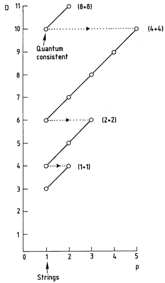
graphics grabbed from (Duff 87)

But there is more: the un-wrapped component of the dimensionally reduced cocycle satisfies the twisted cocycle condition

$$d \, \mu^d_{(p+1)+2} \;=\; mu^d_{p+2} \wedge \mu^d_{0+2} \,.$$

These relations are not to be ignored.

This we turn to now.

$\,$

Dualities

$\,$

We discuss now how

by repeatedly applying

the super $L_\infty$-algebraic dimensional reduction/oxidation isomorphism of prop.

to the descended cocycles (above) from the brane bouquet

yields super $L_\infty$-algebraic equivalences

that reflect the pertinent dualities in string theory

1. between M-theory and type IIA string theory by KK-compactification

2. between type IIA string theory and type IIB string theory (T-duality)

3. between type IIB string theory and itself (S-duality)

4. between type IIB string theory and F-theory.

$\,$

$\,$

We now discuss each aspect of this picture.

$\,$

M/IIA-Duality via Double dimensional reduction via Cyclification

$\,$

The M2-brane/M5-brane in 11d

is all controled by the following Fierz identities

for the $\mathbf{32}$ Majorana spin representation for $Spin(10,1)$

$\,$

$$\left( \overline{\psi} \wedge \Gamma_{a b} \psi \right) \wedge \left( \overline{\psi} \wedge \Gamma^b \psi \right) \;= \; 0 \,.$$

$\,$

and

$\,$

$$\left( \overline{\psi} \wedge \Gamma_{a_1 \cdots a_4 b} \psi \right) \wedge \left( \overline{\psi} \wedge \Gamma^{b} \psi \right) \;=\; 3 \left( \overline{\psi} \Gamma_{[a_1 a_2} \psi \right) \wedge \left( \overline{\psi} \Gamma_{a_3 a_4]} \psi \right)$$

(D’Auria-Fré 82b (3.13) and (3.28))

$\,$

$\,$

The first Fierz identity says that

$$\mu_{M2} \:\coloneqq\; \left( \tfrac{i}{2} \overline{\psi} \wedge \Gamma_{a b} \psi \right) \wedge e^{a} \wedge e^b$$

is a 4-cocycle on $\mathbb{R}^{10,1\vert \mathbf{32}}$, classifying the

supergravity Lie 3-algebra extension

$$\array{ \mathfrak{m}2\mathfrak{brane} \\ \downarrow \\ \mathbb{R}^{10,1\vert \mathbf{32}} } \;\;\;\;\;\;\;\;\; CE(\mathfrak{m}2\mathfrak{brane}) = \left\{ \array{ d \, e^a = \overline{\psi} \wedge \Gamma^a \psi \\ d \, \psi^\alpha = 0 \\ d \, h_3 = \mu_{M2} } \right\}$$

The second says that

$$\mu_{M5} \;\coloneqq\; \tfrac{1}{5!} \left( \overline{\psi} \wedge \Gamma_{a_1 \cdots a_5} \psi \right) \wedge e^{a_1} \wedge \cdots \wedge e^{a_5} \;-\; \tfrac{1}{2} h_3 \wedge \mu_{M2}$$

is a 7-cocycle on $\mathfrak{m}2\mathfrak{brane}$

$$\mu_{M5} \;\colon\; \mathfrak{m}2\mathfrak{brane} \longrightarrow b^6 \mathbb{R}$$

$\,$

Equivalently, (by the discussion at M-Flux fields above)

with $\mathfrak{l}(S^4)$ the rational 4-sphere

$$CE(\mathfrak{l}(S^4)) = \left\{ \array{ d \, g_4 = 0 \\ d \, g_7 = -\tfrac{1}{2} g_4 \wedge g_4 } \right\}$$

then the two Fierz identities together say that there is a single 4-sphere valued cocycle

$$\mu_{M2/M5} \;\colon\; \mathbb{R}^{10,1\vert \mathbf{32}} \longrightarrow \mathfrak{l}(S^4)$$

Hence $S^4$ is the rational coefficient for the unified M2/M5 M-flux fields.

Now we compute what becomes of this under double dimensional reduction via $L_\infty$-cyclification (prop. )

Example

Let $X = S^4$ be the 4-sphere.

Its free loop algebra $\mathcal{L}S^4$ is given by

$$CE( \; \mathfrak{L}S^4 \; ) \;=\; \left\{ \array{ d\, h_3 & = 0 \\ d\, \omega_4 & = 0 \\ d\, \omega_6 & = h_3 \wedge \omega_4 \\ d\, h_7 & = -\tfrac{1}{2} \omega_4 \wedge \omega_4 \\ } \right\}$$

and its cyclification $\mathcal{L}S^4 / S^1$ is given by

$$CE( \; \mathfrak{L}S^4 / \mathbb{R} \; ) \;=\; \left\{ \array{ d \, h_3 & = 0 \\ d \, \omega_2 & = 0 \\ d \, \omega_4 & = h_3 \wedge \omega_2 \\ d \, \omega_6 & = h_3 \wedge \omega_4 \\ d \, h_7 & = -\tfrac{1}{2} \omega_4 \wedge \omega_4 + \omega_2 \wedge \omega_6 } \right. \,.$$

$\,$

$\,$

Proposition

(Fiorenza-Sati-Schreiber 16a, section 3)

The cyclification of the M-brane coefficient $\mathfrak{l}(S^4)$

is the truncated IIA F1/D-brane coefficient $\mathfrak{l}( KU\langle 0,6 \rangle ( B U(1) )$

with an extra twist for the NS5-brane:

$$CE\left( \mathfrak{L} S^4 / \mathbb{R} \right) \;\simeq\; CE\left(\, \underset{\text{F1/Dp-branes}}{\underbrace{ \mathfrak{l}(KU\langle 0,6\rangle/B U(1)) }} \, \right) \underset{\text{NS5-brane}}{\underbrace{ [h_7]/(d h_7 = \omega_2 \wedge \omega_6 - \omega_4 \wedge \omega_4) }} \,.$$

Under this identification

the $L_\infty$-theoretic dimensional reduction according to prop.

of the unified M-brane cocycle $\mu_{M2/M5}$ of prop.

along the M-theory extension from example

is the unified type IIA F1/D-brane cocycle from prop. :

$$\array{ 11d, N = 1 &&&& \mathbb{R}^{10,1\vert \mathbf{32}} && \overset{\mu_{M2/M5}}{\longrightarrow} && \mathfrak{l}(S^4) \\ && && \downarrow \\ 10d, \text{type IIA} && && \mathbb{R}^{9,1\vert \mathbf{16}+ \overline{\mathbf{16}}} && \overset{ { \mathfrak{L}(\mu_{M2/M5})/\mathbb{R} } \atop { = \atop { \mu^{IIA}_{F1/D0/D2/D4/NS5} } } }{\longrightarrow} && { { \mathfrak{l}(\mathcal{L}S^4/S^1) } } \\ && && & {}_{ \mathllap{\mu^{IIA}}_{F1/D0/D2/D4} } \searrow & & \swarrow_{\mathrlap{\text{project out} \atop \text{NS5-coefficient}}} \\ && && && \mathfrak{l}( KU\langle 0,6\rangle/B U(1) ) }$$

$\,$

Observe that (by adjunction) this double dimensional reduction operation

is an isomorphism, hence

• the M2/M5-brane cocycle $\mathbb{R}^{10,1\vert \mathbf{32}} \longrightarrow \mathfrak{l}(S^4)$ in 11d

is equivalent to

• the F1/D$p$/NS5-brane cocycle $\mathbb{R}^{9,1 \vert \mathbf{16} + \overline{\mathbf{16}}} \longrightarrow \mathfrak{l}(\mathcal{L}S^4/S^1)$

Hence this is the M/IIA duality

on super $p$-brane super Lie $n$-algebra cocycles.

$\,$

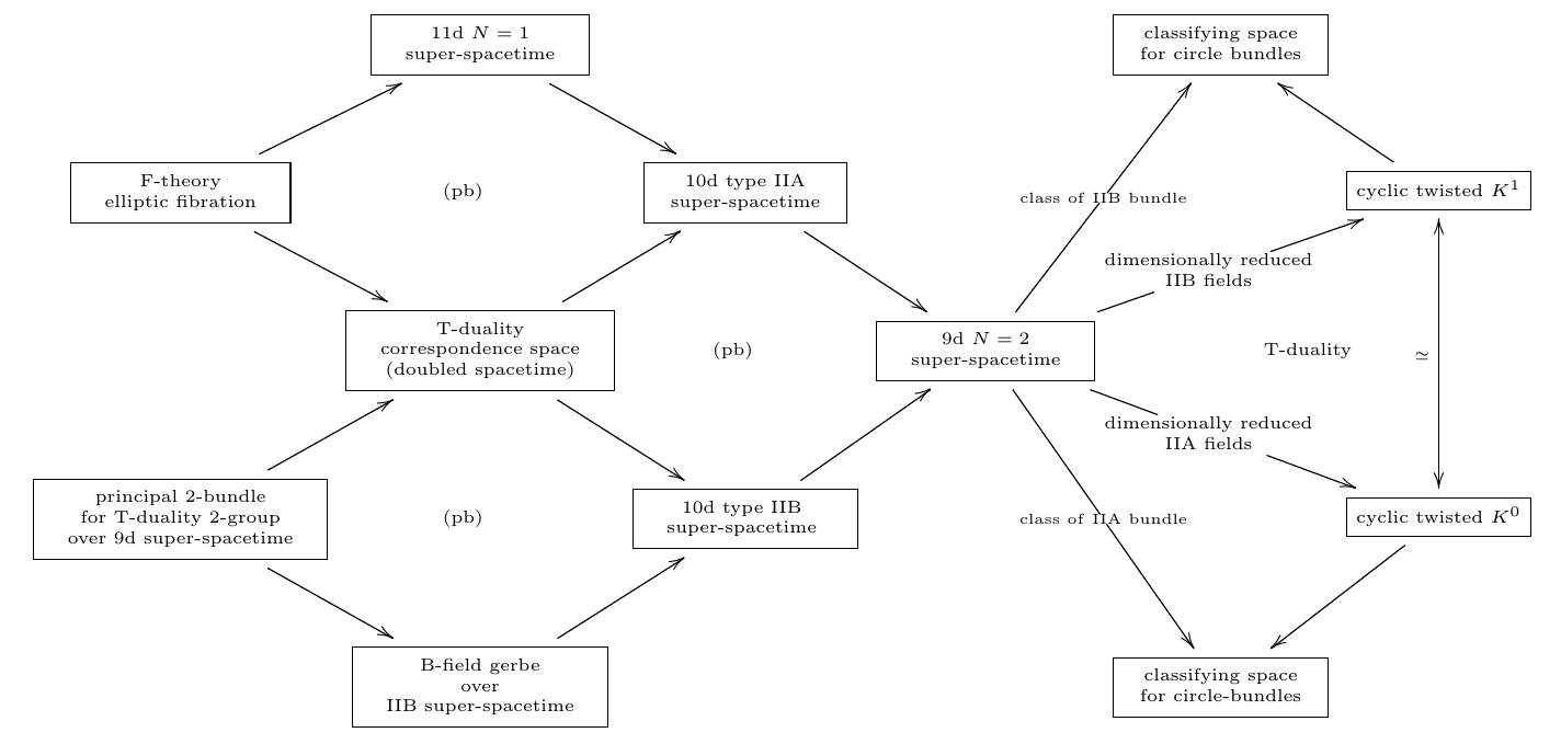
IIA/IIB-Duality via T-Duality

The archetypical duality in string theory is T-duality, which relates the F1/Dp/NS5-super p-branes of type IIA string theory on a superspacetime which is a circle fiber bundle over a 9d base to those of type IIB string theory on a dual circle fibration with the fiber size inverted in string length units. The F1/Dp-super p-brane charges on both sides of this duality take values in twisted K-theory, and hence the mathematical statement here is that dual circle fibrations of this form induce an equivalence in twisted K-theory. This T-duality equivalence of F1/D$p$-brane charges in twisted K-theory is known in the literature as “topological T-duality”.

$\,$

The IIA and the IIB spacetime both extend the single $N = 2$ 9d spacetime

$$\array{ \mathbb{R}^{9,1\vert \mathbf{16} + \mathbf{16}} && && \mathbb{R}^{9,1\vert \mathbf{16} + \overline{\mathbf{16}}} \\ & \searrow && \swarrow \\ && \mathbb{R}^{8,1\vert \mathbf{16} + \mathbf{16}} }$$

Apply double dimensional reduction of the unified $F1/Dp$-cocycles

in IIA and IIB along both of these.

The resulting cyclified $L_\infty$-cocycles in 9d turn out to be $L_\infty$-equivalent.

(FSS16b, sections 5 and 6)

One derives the following picture

$\,$

$\,$

(…)

$\,$

IIB/F

(…)

FSS16b, section 7

(…)

$\,$

$\,$

References

Detailed pointers to the literature are contained in the above text.

Here we only list the references to the original work reported on here.

$\,$

The bosonic string Lie 2-algebra is discussed in the appendix of

• John Baez, Alissa Crans, Urs Schreiber, Danny Stevenson, From loop groups to 2-groups, Homology Homotopy Appl. Volume 9, Number 2 (2007), 101-135. (arXiv:math/0504123)

Its role in Green-Schwarz anomaly cancellation is discussed in

• Hisham Sati, Urs Schreiber, Jim Stasheff, Twisted Differential String and Fivebrane Structures, Communications in Mathematical Physics, Volume 315, Issue 1 (2012) (arXiv:0910.4001)

and its role in the flux quantization of the supergravity C-field in

• Domenico Fiorenza, Hisham Sati, Urs Schreiber, The moduli 3-stack of the C-field, Communications in Mathematical Physics, Volume 333, Issue 1 (2015), Page 117-151 (arXiv:1202.2455)

and

• Domenico Fiorenza, Hisham Sati, Urs Schreiber, Multiple M5-branes, String 2-connections, and 7d nonabelian Chern-Simons theory, Advances in Theoretical and Mathematical Physics, Volume 18, Number 2 (2014) (arXiv:1201.5277)

Our discussion of L-infinity algebra cohomology is due to

• Hisham Sati, Urs Schreiber, Jim Stasheff, L-infinity algebra connections and applications to String- and Chern-Simons n-transport, in Quantum Field Theory, Birkhäuser (2009) 303-424 (arXiv:0801.3480)

The observation of the brane bouquet in super $L_\infty$-algebra and the general construction of higher WZW terms from higher $L_\infty$-cocycles is due to

• Domenico Fiorenza, Hisham Sati, Urs Schreiber, Super Lie n-algebra extensions, higher WZW models and super p-branes with tensor multiplet fields International Journal of Geometric Methods in Modern Physics Volume 12, Issue 02 (2015) 1550018, (arXiv:1308.5264)

The homotopy-descent of the M5-brane cocycle and of the type IIA D-brane cocycles is due to

• Domenico Fiorenza, Hisham Sati, Urs Schreiber, The WZW term of the M5-brane and differential cohomotopy, J. Math. Phys. 56, 102301 (2015) (arXiv:1506.07557)

• Domenico Fiorenza, Hisham Sati, Urs Schreiber, Rational sphere valued supercocycles in M-theory, Journal of Geometry and Physics, Volume 114 (2017) (arXiv:1606.03206)

The derivation of supersymmetric topological T-duality, rationally, and of the higher super Cartan geometry for super T-folds is due to

• Domenico Fiorenza, Hisham Sati, Urs Schreiber, T-Duality from super Lie n-algebra cocycles for super p-branes, ATMP 22 5 (2018) [arXiv:1611.06536]

The derivation of the process of higher invariant extensions that leads from the superpoint to 11-dimensional supergravity:

• John Huerta, Urs Schreiber, M-Theory from the Superpoint

General discussion of twisted cohomology is in

• Thomas Nikolaus, Urs Schreiber, Danny Stevenson, Principal ∞-bundles – General theory, Journal of Homotopy and Related Structures, Volume 10, Issue 4 (2015) (arXiv:1207.0248)

A textbook account of much of the story is in

• Urs Schreiber, differential cohomology in a cohesive topos, Thesis