nLab Introduction to Topological K-Theory

$\,$

These notes give an introduction to topological K-theory, of the basic definitions and results, for readers with a basic knowledge of (point-set) topology. The material covered is largely that also found in Hatcher or Wirthmuller 12.

under construction

Idea

To recall, the subject of topology studies spaces with continuous functions between them: topological spaces, a fundamental concept in all of mathematics. For many applications one cares about the choice of continuous functions only up to continuous deformations, called homotopies. The study of topological spaces with continuous functions up to homotopy is called homotopy theory. Interestingly, this plays an even more fundamental role in mathematics. For some introductory exposition see at Higher Structures in Mathematics and Physics.

In order to study topological spaces up to homotopy – then called homotopy types – a useful strategy is to assign algebraic data to them which may be transferred along continuous functions but is invariant under homotopy: homotopy invariants. This approach to homotopy theory is called algebraic topology.

A basic example of such a homotopy invariant of topological spaces is singular homology and singular cohomology. These are sequences of abelian groups which classify formal formal linear combinations of “singular chains” in a topological space, essentially a simple algebraic way to detect which kind of “holes” there are in a topological space.

But there are more interesting and richer homotopy invariants of topological spaces. In a sense the next example after the “ordinary” singular cohomology is the “generalized cohomology theory” called topological K-theory.

In topological K-theory one detects properties of topological spaces by regarding vector bundles over them. A vector bundle over a topological space $X$ is an assignment of a vector space $V_x$ (the “fiber” over $x$) to each of its points $x \in X$, such that these glue together to one big space $V$ over $X$ as the point $x$ varies in $X$. Hence vector bundles are to be thought of as “continuously varying families of vector spaces”, combining topology with linear algebra.

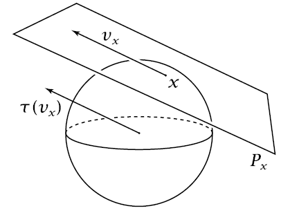
graphics grabbed from Hatcher

For example if $X$ is differentiable, then at each of its points there is a vector space of tangent vectors called the tangent space at that point. The collection of these tangent spaces forms a vector bundle called the tangent bundle. The graphics on the right shows one tangent space to the 2-sphere.

Just as two vector spaces may be combined in their direct sum, so two vector bundles may be combined by point-wise direct sum of their fibers. This makes the isomorphism classes of vector bundles over a fixed topological space form a semi-group (in fact a monoid). The key idea of topological K-theory is to turn this semi-group of vector bundles into an actual (abelian) group by adjoining inverses, a general procudure known as the Grothendieck group construction, after its inventor. Applied to the semi-group of isomorphism classes of vector bundles, this yields the abelian group that is called the topological K-theory group of the underlying topological space. Here the “K” refers to the passage to (isomorphism) classes (German: Klassen).

Topological K-theory studies isomorphism classes of vector bundles over topological spaces together with their formal inverses with respect to direct sum of vector bundles.

$\,$

We now say some of this again, at a slightly more technical level.

$\,$

Recall that for $k$ a field then a $k$-vector bundle over a topological space $X$ is a map $V \to X$ whose fibers are vector spaces which vary over $X$ in a controlled way. Explicitly this means that there exits an open cover $\{U_i \to X\}$ of $X$, a natural number $n \in \mathbb{N}$ (the rank of the vector bundle) and a homeomorphism $U_i \times k^n \to V|_{U_i}$ over $U_i$ which is fiberwise a $k$-linear map.

Vector bundles are of central interest in large parts of mathematics and physics, for instance in Chern-Weil theory and cobordism theory. But the collection $Vect(X)_{/\sim}$ of isomorphism classes of vector bundles over a given space is in general hard to analyze. One reason for this is that these are classified in degree-1 nonabelian cohomology with coefficients in the (nonabelian) general linear group $GL(n,k)$. K-theory may roughly be thought of as the result of forcing vector bundles to be classified by an abelian cohomology theory.

To that end, observe that all natural operations on vector spaces generalize to vector bundles by applying them fiber-wise. Notably there is the fiberwise direct sum of vector bundles, also called the Whitney sum operation. This operation gives the set $Vect(X)_{/\sim}$ of isomorphism classes of vector bundles the structure of an semi-group (monoid) $(Vect(X)_{/\sim},\oplus)$.

Now as under direct sum, the dimension of vector spaces adds, similarly under direct sum of vector bundles their rank adds. Hence in analogy to how one passes from the additive semi-group (monoid) of natural numbers to the addtitive group of integers by adjoining formal additive inverses, so one may adjoin formal additive inverses to $(Vect(X)_{/\sim},\oplus)$. By a general prescription (“Grothendieck group”) this is achieved by first passing to the larger class of pairs $(V_+,V_-)$ of vector bundles (“virtual vector bundles”), and then quotienting out the equivalence relation given by

$$(V_+, V_-) \sim (V_+ \oplus W , V_- \oplus W)$$

for all $W \in Vect(X)_{/\sim}$. The resulting set of equivalence classes is an abelian group with group operation given on representatives by

$$[V_+, V_-] \oplus [V'_+, V'_-] \coloneqq (V_+ \oplus V'_+, V_- \oplus V'_-)$$

and with the inverse of $[V_+,V_-]$ given by

$$-[V_+, V_-] = [V_-, V_+] \,.$$

This abelian group obtained from $(Vect(X)_{/\sim}, \oplus)$ is denoted $K(X)$ and often called the K-theory of the space $X$. Here the letter “K” (due to Alexander Grothendieck) originates as a shorthand for the German word Klasse, referring to the above process of forming equivalence classes of (isomorphism classes) of vector bundles.

This simple construction turns out to yield remarkably useful groups of homotopy invariants. A variety of deep facts in algebraic topology have fairly elementary proofs in terms of topolgical K-theory, for instance

• the proof of topological invariance of dimension;

• the solution of the Hopf invariant one problem (Adams-Atiyah 66),

These proofs make use of the Adams operations on K-theory, which are reflections of the fact that with every vector bundle there is also the exterior tensor powers.

One defines the “higher” K-groups of a topological space to be those of its higher suspensions

$$K^{-n}(X) = K(\Sigma^n X) \,.$$

The assignment $X \mapsto K^\bullet(X)$ turns out to share many properties of the assignment of ordinary cohomology groups $X \mapsto H^n(X,\mathbb{Z})$. One says that topological K-theory is a generalized (Eilenberg-Steenrod) cohomology theory. As such it is represented by a spectrum. For $k = \mathbb{C}$ this is called KU, for $k = \mathbb{R}$ this is called KO. (There is also the unification of both in KR-theory.)

One of the basic facts about topological K-theory, rather unexpected from the definition, is that these higher K-groups repeat periodically in the degree $n$. For $k = \mathbb{R}$ the periodicity is 8, for $k = \mathbb{C}$ it is 2. This is called Bott periodicity. This closely connects to similar periodicities encountered elsewhere in mathematics, notably the periodicity, up to Morita equivalence, of Clifford algebras.

It turns out that an important source of virtual vector bundles representing classes in K-theory are index bundles: Given a Riemannian spin manifold $B$, then there is a vector bundle $S \to B$ called the spin bundle of $B$, which carries a differential operator, called the Dirac operator $D$. The index of a Dirac operator is the formal difference of its kernel by its cokernel $[ker D, coker D]$. Now given a continuous family $D_x$ of Dirac operators/Fredholm operators, parameterized by some topological space $X$, then these indices combine to a class in $K(X)$.

It is via this construction that topological K-theory connects to spin geometry (see e.g. Karoubi K-theory) and index theory.

As the terminology indicates, both spin geometry and Dirac operator originate in physics. Accordingly, K-theory plays a central role in various areas of mathematical physics, for instance in the theory of geometric quantization (“spin^c quantization”) in the theory of D-branes (where it models D-brane charge and RR-fields) and in the theory of Kaluza-Klein compactification via spectral triples (see below).

All these geometric constructions have an operator algebraic incarnation: by the topological Serre-Swan theorem then vector bundles of finite rank are equivalently modules over the C*-algebra of continuous functions on the base space. Using this relation one may express K-theory classes entirely operator algebraically, this is called operator K-theory. Now Dirac operators are generalized to Fredholm operators.

There are more C*-algebras than arising as algebras of functions of topological space, namely non-commutative C-algebras. One may think of these as defining non-commutative geometry, but the definition of operator K-theory immediately generalizes to this situation (see also at KK-theory).

While the C*-algebra of a Riemannian spin manifold remembers only the underlying topological space, one may algebraically encode the smooth structure and Riemannian structure by passing from Fredholm modules to “spectral triples”. This may for instance be used to algebraically encode the spin physics underlying the standard model of particle physics and operator K-theory plays a crucial role in this.

Ordinary cohomology

Idea

We are concerned with assigning abelian groups to topological spaces that tell us something about the nature of these spaces, about their “homotopy type”. Before we come to K-theory, the simplest such assignment is called ordinary homology and ordinary cohomology. In its realization as singular chain homology it uses a basic tool of homological algebra to compute these group: chain complexes.

Consider an interval in a topological space $X$, namely a continuous map $\sigma \colon [0,1] \to X$. Its boundary is the two endpoints $\sigma(0) \colon \ast \to X$ and $\sigma(1) \colon \ast to X$. In order to remember that the first is the “incoming boundary” while the second is the “outgoing boundary” we form their formal difference and call this the oriented boundary

$$\partial \sigma \;\coloneqq\; \sigma(1) - \sigma(0) \,.$$

This suggests that we also allow for signed formal sums $\underset{i}{\sum} a_i \sigma_i$ of intervals in the first place.{ If all these intervals $\sigma_i$ touch each other at their endpoints, then this looks like a chain of intervals, a 1-dimensional chain, and hence such a formal sum is called a 1-chain, for short. Similarly a formal sum of points is then called a 0-chain. It is natural to extend the boundary operation $\partial$ linearly from intervals to 1-chains. The quotient group

$$H_0(X) \coloneqq \frac{\text{0-chains}}{\text{boundaries of 1-chains}}$$

is called the ordinary homology or singular homology of $X$ in degree 0. Clearly, it is measure for the connected components of $X$. Similarly there are $n$-dimensional chains in $X$, for any $n$, and a boundary map $\partial$ on all of these. It satisfies the fundamental identity that The boundary of a boundary vanishes,

$$\partial \circ \partial = 0 \,.$$

One says that the chains equipped with this nilpotent boundary operation form a chain complex. In general then the quotient group

$$H_n(X) \coloneqq \frac{n\text{-chains that are cycles}}{\text{boundaries of}\; n+1\text{-chains}}$$

is called the ordinary homology of $X$ in degree $n$. This a measure for the “holes of dimension $n$” that one may fund in $X$.

The ordinary homólogy groups associated with a topological space are homotopy invariants that are useful for analyzing, recognizing and and distinguishing topological spaces.

Homotopy type of topological spaces

This section reviews some basic notions in topology and homotopy theory. These will all serve as blueprints for corresponding notions in homological algebra.

Definition

A topological space is a set $X$ equipped with a set of subsets $U \subset X$, called open sets, which are closed under

1. finite intersections
2. arbitrary unions.

Example

The Cartesian space $\mathbb{R}^n$ with its standard notion of open subsets given by unions of open balls $D^n \subset \mathbb{R}^n$.

Definition

For $Y \hookrightarrow X$ an injection of sets and $\{U_i \subset X\}_{i \in I}$ a topology on $X$, the subspace topology on $Y$ is $\{U_i \cap Y \subset Y\}_{i \in I}$.

Definition

For $n \in \mathbb{N}$, the topological n-simplex is, up to homeomorphism, the topological space whose underlying set is the subset

$$\Delta^n \coloneqq \{ \vec x \in \mathbb{R}^{n+1} | \sum_{i = 0 }^n x_i = 1 \; and \; \forall i . x_i \geq 0 \} \subset \mathbb{R}^{n+1}$$

of the Cartesian space $\mathbb{R}^{n+1}$, and whose topology is the subspace topology induces from the canonical topology in $\mathbb{R}^{n+1}$.

Example

For $n = 0$ this is the point, $\Delta^0 = *$.

For $n = 1$ this is the standard interval object $\Delta^1 = [0,1]$.

For $n = 2$ this is the filled triangle.

For $n = 3$ this is the filled tetrahedron.

Definition

A homomorphisms between topological spaces $f : X \to Y$ is a continuous function:

a function $f:X\to Y$ of the underlying sets such that the preimage of every open set of $Y$ is an open set of $X$.

Topological spaces with continuous maps between them form the category Top.

Definition

For $n \in \mathbb{N}$, $\n \geq 1$ and $0 \leq k \leq n$, the $k$th $(n-1)$-face (inclusion) of the topological $n$-simplex, def. , is the subspace inclusion

$$\delta_k : \Delta^{n-1} \hookrightarrow \Delta^n$$

induced under the coordinate presentation of def. , by the inclusion

$$\mathbb{R}^n \hookrightarrow \mathbb{R}^{n+1}$$

which “omits” the $k$th canonical coordinate:

$$(x_0, \cdots , x_{n-1}) \mapsto (x_0, \cdots, x_{k-1} , 0 , x_{k}, \cdots, x_{n-1}) \,.$$

Example

The inclusion

$$\delta_0 : \Delta^0 \to \Delta^1$$

is the inclusion

$$\{1\} \hookrightarrow [0,1]$$

of the “right” end of the standard interval. The other inclusion

$$\delta_1 : \Delta^0 \to \Delta^1$$

is that of the “left” end $\{0\} \hookrightarrow [0,1]$.

Definition

For $n \in \mathbb{N}$ and $0 \leq k \lt n$ the $k$th degenerate $(n)$-simplex (projection) is the surjective map

$$\sigma_k : \Delta^{n} \to \Delta^{n-1}$$

induced under the barycentric coordinates of def. under the surjection

$$\mathbb{R}^{n+1} \to \mathbb{R}^n$$

which sends

$$(x_0, \cdots, x_n) \mapsto (x_0, \cdots, x_{k} + x_{k+1}, \cdots, x_n) \,.$$

Definition

For $X \in$ Top and $n \in \mathbb{N}$, a singular $n$-simplex in $X$ is a continuous map

$$\sigma : \Delta^n \to X$$

from the topological $n$-simplex, def. , to $X$.

Write

$$(Sing X)_n \coloneqq Hom_{Top}(\Delta^n , X)$$

for the set of singular $n$-simplices of $X$.

As $n$ varies, this forms the singular simplicial complex of $X$. This is the topic of the next section, see def. def. .

Definition

For $f,g : X \to Y$ two continuous functions between topological spaces, a left homotopy $\eta : f \Rightarrow g$ is a commuting diagram in Top of the form

$$\array{ X \\ {}^{\mathllap{(id,\delta_0)}}\downarrow & \searrow^{\mathrlap{f}} \\ X \times \Delta^1 &\stackrel{\eta}{\to}& Y \\ {}^{\mathllap{(id,\delta_1)}}\uparrow & \nearrow_{\mathrlap{g}} \\ X } \,.$$

Remark

In words this says that a homotopy between two continuous functions $f$ and $g$ is a continuous 1-parameter deformation of $f$ to $g$. That deformation parameter is the canonical coordinate along the interval $[0,1]$, hence along the “length” of the cylinder $X \times \Delta^1$.

Proposition

Left homotopy is an equivalence relation on $Hom_{Top}(X,Y)$.

The fundamental invariants of a topological space in the context of homotopy theory are its homotopy groups. We first review the first homotopy group, called the fundamental group of $X$:

Definition

For $X$ a topological space and $x : * \to X$ a point. A loop in $X$ based at $x$ is a continuous function

$$\gamma : \Delta^1 \to X$$

from the topological 1-simplex, such that $\gamma(0) = \gamma(1) = x$.

A based homotopy between two loops is a homotopy

$$\array{ \Delta^1 \\ \downarrow^{\mathrlap{(id,\delta_0)}} & \searrow^{\mathrlap{f}} \\ \Delta^1 \times \Delta^1 &\stackrel{\eta}{\to}& X \\ \uparrow^{\mathrlap{(id,\delta_1)}} & \nearrow_{\mathrlap{g}} \\ \Delta^1 }$$

such that $\eta(0,-) = \eta(1,-) = x$.

Proposition

This notion of based homotopy is an equivalence relation.

Proof

This is directly checked. It is also a special case of the general discussion at homotopy.

Definition

Given two loops $\gamma_1, \gamma_2 : \Delta^1 \to X$, define their concatenation to be the loop

$$\gamma_2 \cdot \gamma_1 : t \mapsto \left\{ \array{ \gamma_1(2 t) & ( 0 \leq t \leq 1/2 ) \\ \gamma_2(2 (t-1/2)) & (1/2 \leq t \leq 1) } \right. \,.$$

Proposition

Concatenation of loops respects based homotopy classes where it becomes an associative, unital binary pairing with inverses, hence the product in a group.

Definition

For $X$ a topological space and $x \in X$ a point, the set of based homotopy equivalence classes of based loops in $X$ equipped with the group structure from prop. is the fundamental group or first homotopy group of $(X,x)$, denoted

$$\pi_1(X,x) \in Grp \,.$$

Example

The fundamental group of the point is trivial: $\pi_1(*) = *$.

Example

The fundamental group of the circle is the group of integers $\pi_1(S^1) \simeq \mathbb{Z}$.

This construction has a fairly straightforward generalizations to “higher dimensional loops”.

Definition

Let $X$ be a topological space and $x : * \to X$ a point. For $(1 \leq n) \in \mathbb{N}$, the $n$th homotopy group $\pi_n(X,x)$ of $X$ at $x$ is the group:

• whose elements are left-homotopy equivalence classes of maps $S^n \to (X,x)$ in $Top^{*/}$;

• composition is given by gluing at the base point (wedge sum) of representatives.

The 0th homotopy group is taken to be the set of connected components.

Example

For $n = 1$ this reproduces the definition of the fundamental group of def. .

The homotopy theory of topological spaces is all controled by the following notion. The abelianization of this notion, the notion of quasi-isomorphism discussed in def. below is central to homological algebra.

Definition

For $X, Y \in$ Top two topological spaces, a continuous function $f : X \to Y$ between them is called a weak homotopy equivalence if

1. $f$ induces an isomorphism of connected components

   $$\pi_0(f) \colon \pi_0(X) \stackrel{\simeq}{\to} \pi_0(Y)$$

   in Set;

2. for all points $x \in X$ and for all $(1 \leq n) \in \mathbb{N}$ $f$ induces an isomorphism on homotopy groups

   $$\pi_n(f,x) \colon \pi_n(X,x) \stackrel{\simeq}{\to} \pi_n(Y,f(x))$$

   in Grp.

What is called homotopy theory is effectively the study of topological spaces not up to isomorphism (here: homeomorphism), but up to weak homotopy equivalence. Similarly, we will see that homological algebra is effectively the study of chain complexes not up to isomorphism, but up to quasi-isomorphism. But this is slightly more subtle than it may seem, in parts due to the following:

Proposition

The existence of a weak homotopy equivalence from $X$ to $Y$ is a reflexive and transitive relation on Top, but it is not a symmetric relation.

Proof

Reflexivity and transitivity are trivially checked. A counterexample to symmetry is the weak homotopy equivalence between the stanard circle and the pseudocircle.

But we can consider the genuine equivalence relation generated by weak homotopy equivalence:

Definition

We say two spaces $X$ and $Y$ have the same (weak) homotopy type if they are equivalent under the equivalence relation generated by weak homotopy equivalence.

Remark

Equivalently this means that $X$ and $Y$ have the same (weak) homotopy type if there exists a zigzag of weak homotopy equivalences

$$X \leftarrow \to\leftarrow \dots \to Y \,.$$

One can understand the homotopy type of a topological space just in terms of its homotopy groups and how they act on each other. (This data is called a Postnikov tower of $X$.) But computing and handling homotopy groups is in general hard, famously so already for the seemingly simple case of the homotopy groups of spheres. Therefore we now want to simplify the situation by passing to a “linear/abelian approximation”.

Simplicial and singular homology

This section discusses how the “abelianization” of a topological space by singular chains gives rise to the notion of chain complexes and their homology.

Above in def. we saw that to a topological space $X$ is associated a sequence of sets

$$(Sing X)_n \coloneqq Hom_{Top}(\Delta^n, X)$$

of singular simplices. Since the topological $n$-simplices $\Delta^n$ from def. sit inside each other by the face inclusions of def.

$$\delta_k : \Delta^{n-1} \to \Delta^{n}$$

and project onto each other by the degeneracy maps, def.

$$\sigma_k : \Delta^{n+1} \to \Delta^n$$

we dually have functions

$$d_k \coloneqq Hom_{Top}(\delta_k, X) : (Sing X)_n \to (Sing X)_{n-1}$$

that send each singular $n$-simplex to its $k$-face and functions

$$s_k \coloneqq Hom_{Top}(\sigma_k,X) : (Sing X)_{n} \to (Sing X)_{n+1}$$

that regard an $n$-simplex as beign a degenerate (“thin”) $(n+1)$-simplex. All these sets of simplices and face and degeneracy maps between them form the following structure.

Definition

A simplicial set $S \in sSet$ is

• for each $n \in \mathbb{N}$ a set $S_n \in Set$ – the set of $n$-simplices;

• for each injective map $\delta_i : \overline{n-1} \to \overline{n}$ of totally ordered sets $\bar n \coloneqq \{ 0 \lt 1 \lt \cdots \lt n \}$

  a function $d_i : S_{n} \to S_{n-1}$ – the $i$th face map on $n$-simplices;

• for each surjective map $\sigma_i : \overline{n+1} \to \bar n$ of totally ordered sets

  a function $\sigma_i : S_{n} \to S_{n+1}$ – the $i$th degeneracy map on $n$-simplices;

such that these functions satisfy the simplicial identities.

Definition

The simplicial identities satisfied by face and degeneracy maps as above are (whenever these maps are composable as indicated):

1. $d_i \circ d_j = d_{j-1} \circ d_i$ if $i \lt j$,

2. $s_i \circ s_j = s_j \circ s_{i-1}$ if $i \gt j$.

3. $d_i \circ s_j = \left\{ \array{ s_{j-1} \circ d_i & if \; i \lt j \\ id & if \; i = j \; or \; i = j+1 \\ s_j \circ d_{i-1} & if i \gt j+1 } \right.$

It is straightforward to check by explicit inspection that the evident injection and restriction maps between the sets of singular simplices make $(Sing X)_\bullet$ into a simplicial set. We now briefly indicate a systematic way to see this using basic category theory, but the reader already satisfied with this statement should jump ahead to the abelianization of $(Sing X)_n$ in prop. below.

Definition

The simplex category $\Delta$ is the full subcategory of Cat on the free categories of the form

$$\begin{aligned} [0] & \coloneqq \{0\} \\ [1] & \coloneqq \{0 \to 1\} \\ [2] & \coloneqq \{0 \to 1 \to 2\} \\ \vdots \end{aligned} \,.$$

Remark

This is called the “simplex category” because we are to think of the object $[n]$ as being the “spine” of the $n$-simplex. For instance for $n = 2$ we think of $0 \to 1 \to 2$ as the “spine” of the triangle. This becomes clear if we don’t just draw the morphisms that generate the category $[n]$, but draw also all their composites. For instance for $n = 2$ we have_

$$[2] = \left\{ \array{ && 1 \\ & \nearrow && \searrow \\ 0 &&\to&& 2 } \right\} \,.$$

Proposition

A functor

$$S : \Delta^{op} \to Set$$

from the opposite category of the simplex category to the category Set of sets is canonically identified with a simplicial set, def. .

Proof

One checks by inspection that the simplicial identities characterize precisely the behaviour of the morphisms in $\Delta^{op}([n],[n+1])$ and $\Delta^{op}([n],[n-1])$.

This makes the following evident:

Example

The topological simplices from def. arrange into a cosimplicial object in Top, namely a functor

$$\Delta^\bullet : \Delta \to Top \,.$$

With this now the structure of a simplicial set on the singular simplices $(Sing X)_\bullet$, def. , is manifest: it is just the nerve of $X$ with respect to $\Delta^\bullet$, namely:

Definition

For $X$ a topological space its simplicial set of singular simplicies (often called the singular simplicial complex)

$$(Sing X)_\bullet : \Delta^{op} \to Set$$

is given by composition of the functor from example with the hom functor of Top:

$$(Sing X) : [n] \mapsto Hom_{Top}( \Delta^n , X ) \,.$$

Remark (aside)

It turns out that homotopy type of the topological space $X$ is entirely captured by its singular simplicial complex $Sing X$ (this is the content of the homotopy hypothesis-theorem).

Now we abelianize the singular simplicial complex $(Sing X)_\bullet$ in order to make it simpler and hence more tractable.

Definition

A formal linear combination of elements of a set $S \in$ Set is a function

$$a : S \to \mathbb{Z}$$

such that only finitely many of the values $a_s \in \mathbb{Z}$ are non-zero.

Identifying an element $s \in S$ with the function $S \to \mathbb{Z}$, which sends $s$ to $1 \in \mathbb{Z}$ and all other elements to 0, this is written as

$$a = \sum_{s \in S} a_s \cdot s \,.$$

In this expression one calls $a_s \in \mathbb{Z}$ the coefficient of $s$ in the formal linear combination.

Remark

For $S \in$ Set, the group of formal linear combinations $\mathbb{Z}[S]$ is the group whose underlying set is that of formal linear combinations, def. , and whose group operation is the pointwise addition in $\mathbb{Z}$:

$$(\sum_{s \in S} a_s \cdot s) + (\sum_{s \in S} b_s \cdot s) = \sum_{s \in S} (a_s + b_s) \cdot s \,.$$

For the present purpose the following statement may be regarded as just introducing different terminology for the group of formal linear combinations:

Proposition

The group $\mathbb{Z}[S]$ is the free abelian group on $S$.

Definition

For $S_\bullet$ a simplicial set, def. , the free abelian group $\mathbb{Z}[S_n]$ is called the group of (simplicial) $n$-chains on $S$.

Definition

For $X$ a topological space, an $n$-chain on the singular simplicial complex $Sing X$ is called a singular $n$-chain on $X$.

This construction makes the sets of simplices into abelian groups. But this allows to formally add the different face maps in the simplicial set to one single boundary map:

Definition

For $S$ a simplicial set, its alternating face map differential in degree $n$ is the linear map

$$\partial : \mathbb{Z}[S_n] \to \mathbb{Z}[S_{n-1}]$$

defined on basis elements $\sigma \in S_n$ to be the alternating sum of the simplicial face maps:

(1)$$\partial \sigma \coloneqq \sum_{k = 0}^n (-1)^k d_k \sigma \,.$$

Proposition

The simplicial identity, def. part (1), implies that the alternating sum boundary map of def. squares to 0:

$$\partial \circ \partial = 0 \,.$$

Proof

By linearity, it is sufficient to check this on a basis element $\sigma \in S_n$. There we compute as follows:

$$\begin{aligned} \partial \partial \sigma & = \partial \left( \sum_{j = 0}^n (-1)^j d_j \sigma \right) \\ & = \sum_{j=0}^n \sum_{i = 0}^{n-1} (-1)^{i+j} d_i d_j \sigma \\ & = \sum_{0 \leq i \lt j \leq n} (-1)^{i+j} d_i d_j \sigma + \sum_{0 \leq j \leq i \lt n} (-1)^{i + j} d_i d_j \sigma \\ & = \sum_{0 \leq i \lt j \leq n} (-1)^{i+j} d_{j-1} d_i \sigma + \sum_{0 \leq j \leq i \lt n} (-1)^{i + j} d_i d_j \sigma \\ & = - \sum_{0 \leq i \leq j \lt n} (-1)^{i+j} d_{j} d_i \sigma + \sum_{0 \leq j \leq i \lt n} (-1)^{i + j} d_i d_j \sigma \\ & = 0 \end{aligned} \,.$$

Here

1. the first equality is (1);

2. the second is (1) together with the linearity of $d$;

3. the third is obtained by decomposing the sum into two summands;

4. the fourth finally uses the simplicial identity def. (1) in the first summand;

5. the fifth relabels the summation index $j$ by $j +1$;

6. the last one observes that the resulting two summands are negatives of each other.

Example

Let $X$ be a topological space. Let $\sigma^1 : \Delta^1 \to X$ be a singular 1-simplex, regarded as a 1-chain

$$\sigma^1 \in C_1(X) \,.$$

Then its boundary $\partial \sigma \in H_0(X)$ is

$$\partial \sigma^1 = \sigma(0) -\sigma(1)$$

or graphically (using notation as for orientals)

$$\partial \left( \sigma(0) \stackrel{\sigma}{\to} \sigma(1) \right) = (\sigma(0)) - (\sigma(1)) \,.$$

In particular $\sigma$ is a 1-cycle precisely if $\sigma(0) = \sigma(1)$, hence precisely if $\sigma$ is a loop.

Let $\sigma^2 : \Delta^2 \to X$ be a singular 2-chain. The boundary is

$$\partial \left( \array{ && \sigma(1) \\ & {}^{\mathllap{\sigma(0,1)}}\nearrow & \Downarrow^{\mathrlap{\sigma}}& \searrow^{\mathrlap{\sigma^{1,2}}} \\ \sigma(0) &&\underset{\sigma(0,2)}{\to}&& \sigma(2) } \right) = \left( \array{ && \sigma(1) \\ & {}^{\mathllap{\sigma(0,1)}}\nearrow & & \\ \sigma(0) } \right) - \left( \array{ && \\ & & & \\ \sigma(0) &\underset{\sigma(0,2)}{\to}& \sigma(2) } \right) + \left( \array{ && \sigma(1) \\ & & & \searrow^{\mathrlap{\sigma^{1,2}}} \\ && && \sigma(2) } \right) \,.$$

Hence the boundary of the boundary is:

$$\begin{aligned} \partial \partial \sigma &= \partial \left( \left( \array{ && \sigma(1) \\ & {}^{\mathllap{\sigma(0,1)}}\nearrow & & \\ \sigma(0) } \right) - \left( \array{ && \\ & & & \\ \sigma(0) &\underset{\sigma(0,2)}{\to}& \sigma(2) } \right) + \left( \array{ && \sigma(1) \\ & & & \searrow^{\mathrlap{\sigma^{1,2}}} \\ && && \sigma(2) } \right) \right) \\ & = \left( \array{ && \\ & & & \\ \sigma(0) } \right) - \left( \array{ && \sigma(1) \\ & & & \\ } \right) - \left( \array{ && \\ & & & \\ \sigma(0) && } \right) + \left( \array{ && \\ & & & \\ && \sigma(2) } \right) + \left( \array{ && \sigma(1) \\ & & & \\ && && } \right) - \left( \array{ && \\ & & & \\ && && \sigma(2) } \right) \\ & = 0 \end{aligned}$$

Definition

For $S$ a simplicial set, we call the collection

1. of abelian groups of chains $C_n(S) \coloneqq \mathbb{Z}[S_n]$, prop. ;

2. and boundary homomorphisms $\partial_n : C_{n+1}(S) \to C_n(X)$, def.

(for all $n \in \mathbb{N}$) the alternating face map chain complex of $S$:

$$C_\bullet(S) = [ \cdots \stackrel{\partial_2}{\to} \mathbb{Z}[S_2] \stackrel{\partial_1}{\to} \mathbb{Z}[S_1] \stackrel{\partial_0}{\to} \mathbb{Z}[S_0] ] \,.$$

Specifically for $S = Sing X$ we call this the singular chain complex of $X$.

This motivates the general definition:

Definition

A chain complex of abelian groups $C_\bullet$ is a collection $\{C_n \in Ab\}_{n}$ of abelian groups together with group homomorphisms $\{\partial_n : C_{n+1} \to C_n\}$ such that $\partial \circ \partial = 0$.

We turn to this definition in more detail in the next section. The thrust of this construction lies in the fact that the chain complex $C_\bullet(Sing X)$ remembers the abelianized fundamental group of $X$, as well as aspects of the higher homotopy groups: in its chain homology.

Definition

For $C_\bullet(S)$ a chain complex as in def. , and for $n \in \mathbb{N}$ we say

• an $n$-chain of the form $\partial \sigma \in C(S)_n$ is an $n$-boundary;

• a chain $\sigma \in C_n(S)$ is an $n$-cycle if $\partial \sigma = 0$

  (every 0-chain is a 0-cycle).

By linearity of $\partial$ the boundaries and cycles form abelian sub-groups of the group of chains, and we write

$$B_n \coloneqq im(\partial_n) \subset C_n(S)$$

for the group of $n$-boundaries, and

$$Z_n \coloneqq ker(\partial_n) \subset C_(S)$$

for the group of $n$-cycles.

Remark

This means that a singular chain is a cycle if the formal linear combination of the oriented boundaries of all its constituent singular simplices sums to 0.

Remark

More generally, for $R$ any unital ring one can form the degreewise free module $R[Sing X]$ over $R$. The corresponding homology is the singular homology with coefficients in $R$, denoted $H_n(X,R)$. This generality we come to below in the next section.

Definition

For $C_\bullet(S)$ a chain complex as in def. and for $n \in \mathbb{N}$, the degree-$n$ chain homology group $H_n(C(S)) \in Ab$ is the quotient group

$$H_n(C(S)) \coloneqq \frac{ker(\partial_{n-1})}{im(\partial_n)} = \frac{Z_n}{B_n}$$

of the $n$-cycles by the $n$-boundaries – where for $n = 0$ we declare that $\partial_{-1} \coloneqq 0$ and hence $Z_0 \coloneqq C_0$.

Specifically, the chain homology of $C_\bullet(Sing X)$ is called the singular homology of the topological space $X$.

One usually writes $H_n(X, \mathbb{Z})$ or just $H_n(X)$ for the singular homology of $X$ in degree $n$.

Remark

So $H_0(C_\bullet(S)) = C_0(S)/im(\partial_0)$.

Example

For $X$ a topological space we have that the degree-0 singular homology

$$H_0(X) \simeq \mathbb{Z}[\pi_0(X)]$$

is the free abelian group on the set of connected components of $X$.

Example

For $X$ a connected, orientable manifold of dimension $n$ we have

$$H_n(X) \simeq \mathbb{Z} \,.$$

The precise choice of this isomorphism is a choice of orientation on $X$. With a choice of orientation, the element $1 \in \mathbb{Z}$ under this identification is called the fundamental class

$$[X] \in H_n(X)$$

of the manifold $X$.

Definition

Given a continuous map $f : X \to Y$ between topological spaces, and given $n \in \mathbb{N}$, every singular $n$-simplex $\sigma : \Delta^n \to X$ in $X$ is sent to a singular $n$-simplex

$$f_* \sigma : \Delta^n \stackrel{\sigma}{\to} X \stackrel{f}{\to} Y$$

in $Y$. This is called the push-forward of $\sigma$ along $f$. Accordingly there is a push-forward map on groups of singular chains

$$(f_*)_n : C_n(X) \to C_n(Y) \,.$$

Proposition

These push-forward maps make all diagrams of the form

$$\array{ C_{n+1}(X) &\stackrel{(f_*)_{n+1}}{\to}& C_{n+1}(Y) \\ \downarrow^{\mathrlap{\partial^X_n}} && \downarrow^{\mathrlap{\partial^Y_n}} \\ C_n(X) &\stackrel{(f_*)_n}{\to}& C_n(Y) }$$

commute.

Proof

It is in fact evident that push-forward yields a functor of singular simplicial complexes

$$f_* : Sing X \to Sing Y \,.$$

From this the statement follows since $\mathbb{Z}[-] : sSet \to sAb$ is a functor.

Therefore we have an “abelianized analog” of the notion of topological space:

Definition

For $C_\bullet, D_\bullet$ two chain complexes, def. , a homomorphism between them – called a chain map $f_\bullet : C_\bullet \to D_\bullet$ – is for each $n \in \mathbb{N}$ a homomorphism $f_n : C_n \to D_n$ of abelian groups, such that $f_n \circ \partial^C_n = \partial^D_n \circ f_{n+1}$:

$$\array{ \vdots && \vdots \\ \downarrow^{\mathrlap{\partial^C_{n+1}}} && \downarrow^{\mathrlap{\partial^D_{n+1}}} \\ C_{n+1} &\stackrel{f_{n+1}}{\to}& D_{n+1} \\ \downarrow^{\mathrlap{\partial^C_n}} && \downarrow^{\mathrlap{\partial^D_n}} \\ C_{n} &\stackrel{f_{n}}{\to}& D_{n} \\ \downarrow^{\mathrlap{\partial^C_{n-1}}} && \downarrow^{\mathrlap{\partial^D_{n-1}}} \\ \vdots && \vdots } \,.$$

Composition of such chain maps is given by degreewise composition of their components. Clearly, chain complexes with chain maps between them hence form a category – the category of chain complexes in abelian groups, – which we write

$$Ch_\bullet(Ab)) \in Cat \,.$$

Accordingly we have:

Proposition

Sending a topological space to its singular chain complex $C_\bullet(X)$, def. , and a continuous map to its push-forward chain map, prop. , constitutes a functor

$$C_\bullet(-) : Top \to Ch_\bullet(Ab)$$

from the category Top of topological spaces and continuous maps, to the category of chain complexes.

In particular for each $n \in \mathbb{N}$ singular homology extends to a functor

$$H_n(-) : Top \to Ab \,.$$

We close this section by stating the basic properties of singular homology, which make precise the sense in which it is an abelian approximation to the homotopy type of $X$. The proof of these statements requires some of the tools of homological algebra that we develop in the later chapters, as well as some tools in algebraic topology.

Proposition

If $f : X \to Y$ is a continuous map between topological spaces which is a weak homotopy equivalence, def, , then the induced morphism on singular homology groups

$$H_n(f) : H_n(X) \to H_n(Y)$$

is an isomorphism.

(A proof (via CW approximations) is spelled out for instance in (Hatcher, prop. 4.21)).

We therefore also have an “abelian analog” of weak homotopy equivalences:

Definition

For $C_\bullet, D_\bullet$ two chain complexes, a chain map $f_\bullet : C_\bullet \to D_\bullet$ is called a quasi-isomorphism if it induces isomorphisms on all homology groups:

$$f_n : H_n(C) \stackrel{\simeq}{\to} H_n(D) \,.$$

In summary: chain homology sends weak homotopy equivalences to quasi-isomorphisms. Quasi-isomorphisms of chain complexes are the abelianized analog of weak homotopy equivalences of topological spaces.

In particular we have the analog of prop. :

Proposition

The relation “There exists a quasi-isomorphism from $C_\bullet$ to $D_\bullet$.” is a reflexive and transitive relation, but it is not a symmetric relation.

Proof

Reflexivity and transitivity are evident. An explicit counter-example showing the non-symmetry is the chain map

$$\array{ \cdots &\to& 0 &\to& \mathbb{Z} &\stackrel{\cdot 2}{\to}& \mathbb{Z} &\to& 0 &\to& \cdots \\ \cdots && \downarrow && \downarrow && \downarrow && \downarrow && \cdots \\ \cdots &\to& 0 &\to& 0 &\to& \mathbb{Z}/2\mathbb{Z} &\to& 0 &\to& \cdots }$$

from the chain complex concentrated on the morphism of multiplication by 2 on integers, to the chain complex concentrated on the cyclic group of order 2.

This clearly induces an isomorphism on all homology groups. But there is not even a non-zero chain map in the other direction, since there is no non-zero group homomorphism $\mathbb{Z}/2\mathbb{Z} \to \mathbb{Z}$.

Accordingly, as for homotopy types of topological spaces, in homological algebra one regards two chain complexes $C_\bullet$, $D_\bullet$ as essentially equivalent – “of the same weak homology type” – if there is a zigzag of quasi-isomorphisms

$$C_\bullet \leftarrow \to \leftarrow \cdots \to D_\bullet$$

between them. This is made precise by the central notion of the derived category of chain complexes. We turn to this below in section Derived categories and derived functors.

But quasi-isomorphisms are a little coarser than weak homotopy equivalences. The singular chain functor $C_\bullet(-)$ forgets some of the information in the homotopy types of topological spaces. The following series of statements characterizes to some extent what exactly is lost when passing to singular homology, and which information is in fact retained.

First we need a comparison map:

Definition

(Hurewicz homomorphism)

For $(X,x)$ a pointed topological space, the Hurewicz homomorphism is the function

$$\Phi : \pi_k(X,x) \to H_k(X)$$

from the $k$th homotopy group of $(X,x)$ to the $k$th singular homology group defined by sending

$$\Phi : (f : S^k \to X)_{\sim} \mapsto f_*[S_k]$$

a representative singular $k$-sphere $f$ in $X$ to the push-forward along $f$ of the fundamental class $[S_k] \in H_k(S^k)$, example .

Proposition

For $X$ a topological space the Hurewicz homomorphism in degree 0 exhibits an isomorphism between the free abelian group $\mathbb{Z}[\pi_0(X)]$ on the set of path connected components of $X$ and the degree-0 singular homlogy:

$$\mathbb{Z}[\pi_0(X)] \simeq H_0(X) \,.$$

Since a homotopy group in positive degree depends on the homotopy type of the connected component of the base point, while the singular homology does not depend on a basepoint, it is interesting to compare these groups only for the case that $X$ is connected.

Proposition

For $X$ a path-connected topological space the Hurewicz homomorphism in degree 1

$$\Phi : \pi_1(X,x) \to H_1(X)$$

is surjective. Its kernel is the commutator subgroup of $\pi_1(X,x)$. Therefore it induces an isomorphism from the abelianization $\pi_1(X,x)^{ab} \coloneqq \pi_1(X,x)/[\pi_1,\pi_1]$:

$$\pi_1(X,x)^{ab} \stackrel{\simeq}{\to} H_1(X) \,.$$

For higher connected $X$ we have the

Theorem

If $X$ is (n-1)-connected for $n \geq 2$ then

$$\Phi : \pi_n(X,x) \to H_n(X)$$

is an isomorphism.

This is known as the Hurewicz theorem.

References

• Allen Hatcher, section 2.1 of Algebraic topology

Vector bundles

Idea

For understanding some topological space $X$, it is often useful to understand how another topological space $F$ may be “continuously distributed over” $X$. For instance the two-element space $\{-1, 1\}$ may be continuously distributed over the circle $S^1$ in two inequivalent ways: Either the two points come back to themselves as we move around the circle, or they switch position. This switch is a reflection of the fact that in the circle there are non-contractible loops, in constrast for instance to the 2-sphere, where every loop may be continuously shrunk to a constant loop. If we embed the two points $\{-1,1\}$ into the real line and repeat the construction, then as the line traces around the circle it sweeps out one of two different topological spaces over the circle: either the cylinder (if $+1$ comes back to itself) or the Möbius strip (if $+1$ and $-1$ change position as one goes around the circle).

The image of this situation looks like a “bundle” of “fibers” over the circle. Generally, for $F$ a topological space, then an $F$-fiber bundle over $X$ is another space $E$ with a projection $p \colon E \to X$ that shrinks the fibers away, which all look like $F$ in a controlled way.

For the purpose of topological K-theory we are interested in fibers $F$ which are vector spaces and such that their re-identification as we move around in $X$ is by linear maps. Then one speaks of vector bundles. The theory of vector bundles is much like “continuously parameterized linear algebra”

Fiber bundles

• fiber bundle

• covering space

• vector bundle

• principal bundle

• associated bundle

The tensor category of vector bundles

• tensor category

category of vector bundles

• direct sum of vector bundles

• tensor product of vector bundles

• dual vector bundle

• pullback bundle

Examples

• Möbius strip

• canonical bundle

• basic line bundle on the 2-sphere

• clutching construction

• universal vector bundle, universal complex line bundle

Basic properties

metric structure

• orthogonal structure

• Hermitian structure

over compact topological spaces

• concordance

• direct summand of trivial bundle

References

• Hatcher, section 1.1

• Wirthmuller 12, section 1 and section 3

Classifying spaces

Idea

Some vector bundles are “tautological”. For consider the topological space of all $k$-dimensional linear subspaces of a fixed $n$-dimensional vector space. Clearly this space carries a vector bundle, namely that whose fiber over the point that labels some subspace is that subspace. It is possible to take this construction and allow $n$ to go to infinity. The result is a classifying space for vector bundles which carries a universal vector bundle: every other vector bundle on a sufficiently well-behaved topological space is classified by a map into this classifying space, namely the map that, roughly, sends each point to the lable of the fiber above it.

classifying spaces for vector bundles.

We use the above fact (…) that

1. every real vector bundle is isomorphic to the canonical associated bundle to an O(n)-principal bundle;

2. every complex vector bundle is isomorphic to the canonical associated bundle to an U(n)-principal bundle.

Grassmannian spaces

In the following we take Top to denote compactly generated topological spaces. For these the Cartesian product $X \times (-)$ is a left adjoint and hence preserves colimits.

Definition

For $n, k \in \mathbb{N}$ and $n \leq k$, then the $n$th real Stiefel manifold of $\mathbb{R}^k$ is the coset topological space.

$$V_n(\mathbb{R}^k) \coloneqq O(k)/O(k-n) \,,$$

where the action of $O(k-n)$ is via its canonical embedding $O(k-n)\hookrightarrow O(k)$.

Similarly the $n$th complex Stiefel manifold of $\mathbb{C}^k$ is

$$V_n(\mathbb{C}^k) \coloneqq U(k)/U(k-n) \,,$$

here the action of $U(k-n)$ is via its canonical embedding $U(k-n)\hookrightarrow U(k)$.

Definition

For $n, k \in \mathbb{N}$ and $n \leq k$, then the $n$th real Grassmannian of $\mathbb{R}^k$ is the coset topological space.

$$Gr_n(\mathbb{R}^k) \coloneqq O(k)/(O(n) \times O(k-n)) \,,$$

where the action of the product group is via its canonical embedding $O(n)\times O(k-n) \hookrightarrow O(n)$ into the orthogonal group.

Similarly the $n$th complex Grassmannian of $\mathbb{C}^k$ is the coset topological space.

$$Gr_n(\mathbb{C}^k) \coloneqq U(k)/(U(n) \times U(k-n)) \,,$$

where the action of the product group is via its canonical embedding $U(n)\times U(k-n) \hookrightarrow U(n)$ into the unitary group.

Example

• $Gr_1(\mathbb{R}^{n+1}) \simeq \mathbb{R}P^n$ is real projective space of dimension $n$.

• $Gr_1(\mathbb{C}^{n+1}) \simeq \mathbb{C}P^n$ is complex projective space of dimension $n$.

Proposition

For all $n \leq k \in \mathbb{N}$, the canonical projection from the real Stiefel manifold (def. ) to the Grassmannian is a $O(n)$-principal bundle

$$\array{ O(n) &\hookrightarrow& V_n(\mathbb{R}^k) \\ && \downarrow \\ && Gr_n(\mathbb{R}^k) }$$

and the projection from the complex Stiefel manifold to the Grassmannian us a $U(n)$-principal bundle:

$$\array{ U(n) &\hookrightarrow& V_n(\mathbb{C}^k) \\ && \downarrow \\ && Gr_n(\mathbb{C}^k) } \,.$$

Proof

By (this cor. and this prop.).

Definition

By def. there are canonical inclusions

$$Gr_n(\mathbb{R}^k) \hookrightarrow Gr_n(\mathbb{R}^{k+1})$$

and

$$Gr_n(\mathbb{C}^k) \hookrightarrow Gr_n(\mathbb{C}^{k+1})$$

for all $k \in \mathbb{N}$. The colimit (in Top, see there) over these inclusions is denoted

$$B O(n) \coloneqq \underset{\longrightarrow}{\lim}_k Gr_n(\mathbb{R}^k)$$

and

$$B U(n) \coloneqq \underset{\longrightarrow}{\lim}_k Gr_n(\mathbb{C}^k) \,,$$

respectively.

Moreover, by def. there are canonical inclusions

$$V_n(\mathbb{R}^k) \hookrightarrow V_n(\mathbb{R}^{k+1})$$

and

$$V_n(\mathbb{C}^k) \hookrightarrow V_n(\mathbb{C}^{k+1}) \,,$$

respectively, that are compatible with the $O(n)$-action and the $U(n)$-action, respectively. The colimit (in Top, see there) over these inclusions, regarded as equipped with the induced action, is denoted

$$E O(n) \coloneqq \underset{\longrightarrow}{\lim}_k V_n(\mathbb{R}^k)$$

and

$$E U(n) \coloneqq \underset{\longrightarrow}{\lim}_k V_n(\mathbb{C}^k) \,,$$

respectively. The inclusions are in fact compatible with the bundle structure from prop. , so that there are induced projections

$$\left( \array{ E O(n) \\ \downarrow \\ B O(n) } \right) \;\; \simeq \;\; \underset{\longrightarrow}{\lim}_k \left( \array{ V_n(\mathbb{R}^k) \\ \downarrow \\ Gr_n(\mathbb{R}^k) } \right)$$

and

$$\left( \array{ E U(n) \\ \downarrow \\ B U(n) } \right) \;\; \simeq \;\; \underset{\longrightarrow}{\lim}_k \left( \array{ V_n(\mathbb{C}^k) \\ \downarrow \\ Gr_n(\mathbb{C}^k) } \right) \,,$$

respectively. These are the standard models for the universal principal bundles for $O$ and $U$, respectively. The corresponding associated vector bundles

$$E O(n) \underset{O(n)}{\times} \mathbb{R}^n$$

and

$$E U(n) \underset{U(n)}{\times} \mathbb{C}^n$$

are the corresponding universal vector bundles.

Since the Cartesian product $O(n)\times (-)$ in compactly generated topological spaces preserves colimits, it follows that the colimiting bundle is still an $O(n)$-principal bundle

$$\begin{aligned} (E O(n))/O(n) & \simeq (\underset{\longrightarrow}{\lim}_k V_{n}(\mathbb{R}^k))/O(n) \\ & \simeq \underset{\longrightarrow}{\lim}_k (V_n(\mathbb{R}^k)/O(n)) \\ & \simeq \underset{\longrightarrow}{\lim}_k Gr_n(\mathbb{R}^k) \\ & \simeq B O(n) \end{aligned}$$

and anlogously for $E U(n)$.

As such this is the standard presentation for the $O(n)$-universal principal bundle. Its base space $B O(n)$ is the corresponding classifying space.

Definition

There are canonical inclusions

$$Gr_n(\mathbb{R}^k) \hookrightarrow Gr_{n+1}(\mathbb{R}^{k+1})$$

and

$$Gr_n(\mathbb{C}^k) \hookrightarrow Gr_{n+1}(\mathbb{C}^{k+1})$$

given by adjoining one coordinate to the ambient space and to any subspace. Under the colimit of def. these induce maps of classifying spaces

$$B O(n) \longrightarrow B O(n+1)$$

and

$$B U(n) \longrightarrow B U(n+1) \,.$$

Definition

There are canonical maps

$$Gr_{n_1}(\mathbb{R}^{k_1}) \times Gr_{n_2}(\mathbb{R}^{k_2}) \longrightarrow Gr_{n_1 + n_2}(\mathbb{R}^{k_1 + k_2})$$

and

$$Gr_{n_1}(\mathbb{C}^{k_1}) \times Gr_{n_2}(\mathbb{C}^{k_2}) \longrightarrow Gr_{n_1 + n_2}(\mathbb{C}^{k_1 + k_2})$$

given by sending ambient spaces and subspaces to their direct sum.

Under the colimit of def. these induce maps of classifying spaces

$$B O(n_1) \times B O(n_2) \longrightarrow B O(n_1 + n_2)$$

and

$$B U(n_1) \times B U(n_2) \longrightarrow B U(n_1 + n_2)$$

Properties

Proposition

The real Grassmannians $Gr_n(\mathbb{R}^k)$ and the complex Grassmannians $Gr_n(\mathbb{C}^k)$ of def. admit the structure of CW-complexes. Moreover the canonical inclusions

$$Gr_n(\mathbb{R}^k) \hookrightarrow Gr_n(\mathbb{R}^{k+1})$$

and

$$Gr_n(\mathbb{C}^k) \hookrightarrow Gr_n(\mathbb{C}^{k+1})$$

are subcomplex incusions (hence relative cell complex inclusions).

Accordingly there is an induced CW-complex structure on the classifying spaces $B O(n)$ and $B U(n)$ (def. ).

A proof is spelled out in (Hatcher, section 1.2 (pages 31-34)).

Proposition

The Stiefel manifold $V_n(\mathbb{R}^k)$ from def. admits the structure of a CW-complex.

e.g. (James 59, p. 3, James 76, p. 5 with p. 21, Blaszczyk 07)

(And I suppose with that cell structure the inclusions $V_n(\mathbb{R}^k) \hookrightarrow V_n(\mathbb{R}^{k+1})$ are subcomplex inclusions.)

Proposition

The Stiefel manifold $V_n(\mathbb{R}^k)$ (def. ) is (k-n-1)-connected.

Proof

Consider the coset quotient projection

$$O(k-n) \longrightarrow O(k) \longrightarrow O(k)/O(k-n) = V_n(\mathbb{R}^k) \,.$$

Since the orthogonal groups is compact (prop.) and by this corollary the projection $O(k)\to O(k)/O(k-n)$ is a Serre fibration. Therefore there is induced the long exact sequence of homotopy groups of this fiber sequence, and by this prop. it has the following form in degrees bounded by $n$:

$$\cdots \to \pi_{\bullet \leq k-n-1}(O(k-n)) \overset{epi}{\longrightarrow} \pi_{\bullet \leq k-n-1}(O(k)) \overset{0}{\longrightarrow} \pi_{\bullet \leq k-n-1}(V_n(\mathbb{R}^k)) \overset{0}{\longrightarrow} \pi_{\bullet-1 \lt k-n-1}(O(k)) \overset{\simeq}{\longrightarrow} \pi_{\bullet-1 \lt k-n-1}(O(k-n)) \to \cdots \,.$$

This implies the claim. (Exactness of the sequence says that every element in $\pi_{\bullet \leq n-1}(V_n(\mathbb{R}^k))$ is in the kernel of zero, hence in the image of 0, hence is 0 itself.)

Similarly:

Proposition

The complex Stiefel manifold $V_n(\mathbb{C}^k)$ (def. ) is 2(k-n)-connected.

Proof

Consider the coset quotient projection

$$U(k-n) \longrightarrow U(k) \longrightarrow U(k)/U(k-n) = V_n(\mathbb{C}^k) \,.$$

By prop. and by this corollary the projection $U(k)\to U(k)/U(k-n)$ is a Serre fibration. Therefore there is induced the long exact sequence of homotopy groups of this fiber sequence, and by prop. it has the following form in degrees bounded by $n$:

$$\cdots \to \pi_{\bullet \leq 2(k-n)}(U(k-n)) \overset{epi}{\longrightarrow} \pi_{\bullet \leq 2(k-n)}(U(k)) \overset{0}{\longrightarrow} \pi_{\bullet \leq 2(k-n)}(V_n(\mathbb{C}^k)) \overset{0}{\longrightarrow} \pi_{\bullet-1 \lt 2(k-n)}(U(k)) \overset{\simeq}{\longrightarrow} \pi_{\bullet-1 \lt 2(k-n)}(U(k-n)) \to \cdots \,.$$

This implies the claim.

Corollary

The colimiting space $E O(n) = \underset{\longrightarrow}{\lim}_k V_n(\mathbb{R}^k)$ from def. is weakly contractible.

The colimiting space $E U(n) = \underset{\longrightarrow}{\lim}_k V_n(\mathbb{C}^k)$ from def. is weakly contractible.

Proposition

The homotopy groups of the classifying spaces $B O(n)$ and $B U(n)$ (def. ) are those of the orthogonal group $O(n)$ and of the unitary group $U(n)$, respectively, shifted up in degree: there are isomorphisms

$$\pi_{\bullet+1}(B O(n)) \simeq \pi_\bullet O(n)$$

and

$$\pi_{\bullet+1}(B U(n)) \simeq \pi_\bullet U(n)$$

(for homotopy groups based at the canonical basepoint).

Proof

Consider the sequence

$$O(n) \longrightarrow E O(n) \longrightarrow B O(n)$$

from def. , with $O(n)$ the fiber. Since (by this prop.) the second map is a Serre fibration, this is a fiber sequence and so it induces a long exact sequence of homotopy groups of the form

$$\cdots \to \pi_\bullet(O(n)) \longrightarrow \pi_\bullet(E O(n)) \longrightarrow \pi_\bullet(B O(n)) \longrightarrow \pi_{\bullet-1}(O (n)) \longrightarrow \pi_{\bullet-1}(E O(n)) \to \cdots \,.$$

Since by cor. $\pi_\bullet(E O(n))= 0$, exactness of the sequence implies that

$$\pi_\bullet(B O(n)) \overset{\simeq}{\longrightarrow} \pi_{\bullet-1}(O (n))$$

is an isomorphism.

The same kind of argument applies to the complex case.

Proposition

For $n \in \mathbb{N}$ there are homotopy fiber sequences

$$S^n \longrightarrow B O(n) \longrightarrow B O(n+1)$$

and

$$S^{2n+1} \longrightarrow B U(n) \longrightarrow B U(n+1) \,,$$

exhibiting the n-sphere ($(2n+1)$-sphere) as the homotopy fiber of the canonical maps from def. .

This means that there is a replacement of the canonical inclusion $B O(n) \hookrightarrow B O(n+1)$ (induced via def. ) by a Serre fibration

$$\array{ B O(n) &\hookrightarrow& B O(n+1) \\ {}^{\mathllap{{weak \, homotopy} \atop equivalence}}\downarrow & \nearrow_{\mathrlap{Serre \, fib.}} \\ \tilde B O(n) }$$

such that $S^n$ is the ordinary fiber of $B O(n)\to \tilde B O(n+1)$, and analogously for the complex case.

Proof

Take $\tilde B O(n) \coloneqq (E O(n+1))/O(n)$.

To see that the canonical map $B O(n)\longrightarrow (E O(n+1))/O(n)$ is a weak homotopy equivalence consider the commuting diagram

$$\array{ O(n) &\overset{id}{\longrightarrow}& O(n) \\ \downarrow && \downarrow \\ E O(n) &\longrightarrow& E O(n+1) \\ \downarrow && \downarrow \\ B O(n) &\longrightarrow& (E O(n+1))/O(n) } \,.$$

By this prop. both bottom vertical maps are Serre fibrations and so both vertical sequences are fiber sequences. By prop. part of the induced morphisms of long exact sequences of homotopy groups looks like this

$$\array{ \pi_\bullet(B O(n)) &\overset{}{\longrightarrow}& \pi_\bullet( (E O(n+1))/O(n) ) \\ {}^{\mathllap{\simeq}}\downarrow && \downarrow^{\mathrlap{\simeq}} \\ \pi_{\bullet-1}(O(n)) &\overset{=}{\longrightarrow}& \pi_{\bullet-1}(O(n)) } \,,$$

where the vertical and the bottom morphism are isomorphisms. Hence also the to morphisms is an isomorphism.

That $B O(n)\to \tilde B O(n+1)$ is indeed a Serre fibration follows again with this prop., which gives the fiber sequence

$$O(n+1)/O(n) \longrightarrow (E O(n+1))/O(n) \longrightarrow (E O(n+1))/O(n+1) \,.$$

The claim in then follows since (this exmpl.)

$$O(n+1)/O(n) \simeq S^n \,.$$

The argument for the complex case is of the same form, concluding now with the identification (this exmpl.)

$$U(n+1)/U(n) \simeq S^{2n+1} \,.$$

The classification result

Proposition

For $X$ a paracompact topological space, the operation of pullback of the universal principal bundle $E O(n) \to B O(n)$ from def. along continuous functions $f \colon X \to B O(n)$ eastblishes a bijection

$$[X, B O(n)] \underoverset{iso}{f \mapsto f^\ast E O(n)}{\longrightarrow} O(n) Bund/_\sim$$

between homotopy classes of functions from $X$ to $B O(n)$ and isomorphism classes of $O(n)$-principal bundles on $X$.

A full proof is spelled out in (Hatcher, section 1.2, theorem 1.16)

References

• Hatcher, section 1.2

• Wirthmuller 12, section 2

• Aguilar-Gitler-Prieto 02, sections 8.3-8-5

The K-theory functor $K^\bullet(-)$

Idea

The isomorphism classes of vector bundles over some topological space $X$ naturally form a semi-group (in fact a monoid) under forming direct sum of vector bundles. But as in ordinary cohomology, we rater want to assign an actual group to $X$, instead of just a semi-group.

There is a universal way to turn a semi-group into an actual group by adjoining formal inverses to all elements. This is called the Grothendieck group construction. Applying this to the semi-group of vector bundles yields “virtual vector bundles”, which are formal differences $[E] - [F]$ of isomorphism classes of actual vector bundles. These now form an abelian group called the topological K-theory group of $X$, and denoted $K(X)$.

Since for every continuous function $f \;\colon\; X \to Y$ and every vector bundle over $Y$ there is the corresponding pullback bundle over $X$, this construction is a (contravariant) functor on the category of topological spaces, just as the ordinary cohomology groups are. In the next session we see that this analogy goes further, so we also call $K(X)$ the K-cohomology group of $X$.

In fact $K(X)$ has more structure than just that of an abelian group. The tensor product of vector bundles makes it a ring. In the next session this will make us say that topological K-theory is a multiplicative cohomology theory.

References

• Wirthmuller 12, sections 6 and 10

• Hatcher, section 2.1

• Aguilar-Gitler-Prieto 02, section 9

Generalized cohomology

Idea

We may now make precise in which sense the topological K-theory functor $K(-)$ is directly analogous to the ordinary cohomology functors $H^\bullet(-,\mathbb{Z})$. This involves noticing a list of useful properties satisfied by these functors. In particular one finds that given any continuous function, then it induces a sequence of further continuous functions called its mapping cones and suspensions, and the application of a cohomology functor to these sequences of topological spaces yields long exact sequences in cohomology. This is most useful for computing generalized cohomology groups.

$\,$

There are two versions of the statement of the axioms:

• Reduced cohomology;

• Unreduced cohomology.

There are functors taking any reduced cohomology theory to an unreduced one, and vice versa. When some fine detail in the axioms is suitably set up, then this establishes an equivalence between reduced and unreduced generalized cohomology:

• Relation between reduced and unreduced cohomology

Mapping cones

• mapping cylinder

• mapping cone

• homotopy cofiber

Reduced cohomology

Throughout, write Top${}_{CW}$ for the category of topological spaces homeomorphic to CW-complexes. Write $Top^{\ast/}_{CW}$ for the corresponding category of pointed topological spaces.

Recall that colimits in $Top^{\ast/}$ are computed as colimits in $Top$ after adjoining the base point and its inclusion maps to the given diagram

Example

The coproduct in pointed topological spaces is the wedge sum, denoted $\vee_{i \in I} X_i$.

Write

$$\Sigma \coloneqq S^1 \wedge (-) \;\colon\; Top^{\ast/}_{CW} \longrightarrow Top^{\ast/}_{CW}$$

for the reduced suspension functor.

Write $Ab^{\mathbb{Z}}$ for the category of integer-graded abelian groups.

Definition

A reduced cohomology theory is a functor

$$\tilde E^\bullet \;\colon\; (Top^{\ast/}_{CW})^{op} \longrightarrow Ab^{\mathbb{Z}}$$

from the opposite of pointed topological spaces (CW-complexes) to $\mathbb{Z}$-graded abelian groups (“cohomology groups”), in components

$$\tilde E \;\colon\; (X \stackrel{f}{\longrightarrow} Y) \mapsto (\tilde E^\bullet(Y) \stackrel{f^\ast}{\longrightarrow} \tilde E^\bullet(X)) \,,$$

and equipped with a natural isomorphism of degree +1, to be called the suspension isomorphism, of the form

$$\sigma \;\colon\; \tilde E^{\bullet +1}(\Sigma -) \overset{\simeq}{\longrightarrow} \tilde E^\bullet(-)$$

such that:

1. (homotopy invariance) If $f_1,f_2 \colon X \longrightarrow Y$ are two morphisms of pointed topological spaces such that there is a (base point preserving) homotopy $f_1 \simeq f_2$ between them, then the induced homomorphisms of abelian groups are equal

   $$f_1^\ast = f_2^\ast \,.$$

2. (exactness) For $i \colon A \hookrightarrow X$ an inclusion of pointed topological spaces, with $j \colon X \longrightarrow Cone(i)$ the induced mapping cone, then this gives an exact sequence of graded abelian groups

   $$\tilde E^\bullet(Cone(i)) \overset{j^\ast}{\longrightarrow} \tilde E^\bullet(X) \overset{i^\ast}{\longrightarrow} \tilde E^\bullet(A) \,.$$

We say $\tilde E^\bullet$ is additive if in addition

• (wedge axiom) For $\{X_i\}_{i \in I}$ any set of pointed CW-complexes, then the canonical comparison morphism

  $$\tilde E^\bullet(\vee_{i \in I} X_i) \longrightarrow \prod_{i \in I} \tilde E^\bullet(X_i)$$

  is an isomorphism, from the functor applied to their wedge sum, example , to the product of its values on the wedge summands, .

We say $\tilde E^\bullet$ is ordinary if its value on the 0-sphere $S^0$ is concentrated in degree 0:

• (Dimension) $\tilde E^{\bullet\neq 0}(\mathbb{S}^0) \simeq 0$.

A homomorphism of reduced cohomology theories

$$\eta \;\colon\; \tilde E^\bullet \longrightarrow \tilde F^\bullet$$

is a natural transformation between the underlying functors which is compatible with the suspension isomorphisms in that all the following squares commute

$$\array{ \tilde E^\bullet(X) &\overset{\eta_X}{\longrightarrow}& \tilde F^\bullet(X) \\ {}^{\mathllap{\sigma_E}}\downarrow && \downarrow^{\mathrlap{\sigma_F}} \\ \tilde E^{\bullet + 1}(\Sigma X) &\overset{\eta_{\Sigma X}}{\longrightarrow}& \tilde F^{\bullet + 1}(\Sigma X) } \,.$$

(e.g. AGP 02, def. 12.1.4)

We may rephrase this more intrinsically and more generally:

Definition

Let $\mathcal{C}$ be an (∞,1)-category with (∞,1)-pushouts, and with a zero object $0 \in \mathcal{C}$. Write $\Sigma \colon \mathcal{C} \to \mathcal{C}\colon X\mapsto 0 \underset{X}{\sqcup} 0$ for the corresponding suspension (∞,1)-functor.

A reduced generalized cohomology theory on $\mathcal{C}$ is

1. a functor

   $$E^\bullet \;\colon \; Ho(\mathcal{C})^{op} \longrightarrow Ab^{\mathbb{Z}}$$

   (from the opposite of the homotopy category of $\mathcal{C}$ into $\mathbb{Z}$-graded abelian groups);

2. a natural isomorphisms (“suspension isomorphisms”) of degree +1

   $$\sigma \; \colon \; H^\bullet \longrightarrow H^{\bullet+1} \circ \Sigma$$

such that $H^\bullet$

1. takes small coproducts to products;

2. takes homotopy cofiber sequences to exact sequences.

Definition

Given a generalized cohomology theory $(H^\bullet,\sigma)$ on some $\mathcal{C}$ as in def. , and given a homotopy cofiber sequence in $\mathcal{C}$

$$X \stackrel{f}{\longrightarrow} Y \stackrel{g}{\longrightarrow} Z \stackrel{coker(g)}{\longrightarrow} \Sigma X \,,$$

then the corresponding connecting homomorphism is the composite

$$\partial \;\colon\; E^\bullet(X) \stackrel{\sigma}{\longrightarrow} E^{\bullet+1}(\Sigma X) \stackrel{coker(g)^\ast}{\longrightarrow} E^{\bullet+1}(Z) \,.$$

Proposition

The connecting homomorphisms of def. are parts of long exact sequences

$$\cdots \stackrel{\partial}{\longrightarrow} E^{\bullet}(Z) \longrightarrow E^\bullet(Y) \longrightarrow E^\bullet(X) \stackrel{\partial}{\longrightarrow} E^{\bullet+1}(Z) \to \cdots \,.$$

Proof

By the defining exactness of $E^\bullet$, def. , and the way this appears in def. , using that $\sigma$ is by definition an isomorphism.

Unreduced cohomology

In the following a pair $(X,A)$ refers to a subspace inclusion of topological spaces (CW-complexes) $A \hookrightarrow X$. Whenever only one space is mentioned, the subspace is assumed to be the empty set $(X, \emptyset)$. Write $Top_{CW}^{\hookrightarrow}$ for the category of such pairs (the full subcategory of the arrow category of $Top_{CW}$ on the inclusions). We identify $Top_{CW} \hookrightarrow Top_{CW}^{\hookrightarrow}$ by $X \mapsto (X,\emptyset)$.

Definition

A cohomology theory (unreduced, relative) is a functor

$$E^\bullet : (Top_{CW}^{\hookrightarrow})^{op} \to Ab^{\mathbb{Z}}$$

to the category of $\mathbb{Z}$-graded abelian groups, as well as a natural transformation of degree +1, to be called the connecting homomorphism, of the form

$$\delta_{(X,A)} \;\colon\; E^\bullet(A, \emptyset) \to E^{\bullet + 1}(X, A) \,.$$

such that:

1. (homotopy invariance) For $f \colon (X_1,A_1) \to (X_2,A_2)$ a homotopy equivalence of pairs, then

   $$E^\bullet(f) \;\colon\; E^\bullet(X_2,A_2) \stackrel{\simeq}{\longrightarrow} E^\bullet(X_1,A_1)$$

   is an isomorphism;

2. (exactness) For $A \hookrightarrow X$ the induced sequence

   $$\cdots \to E^n(X, A) \longrightarrow E^n(X) \longrightarrow E^n(A) \stackrel{\delta}{\longrightarrow} E^{n+1}(X, A) \to \cdots$$

   is a long exact sequence of abelian groups.

3. (excision) For $U \hookrightarrow A \hookrightarrow X$ such that $\overline{U} \subset Int(A)$, then the natural inclusion of the pair $i \colon (X-U, A-U) \hookrightarrow (X, A)$ induces an isomorphism

   $$E^\bullet(i) \;\colon\; E^n(X, A) \overset{\simeq}{\longrightarrow} E^n(X-U, A-U)$$

We say $E^\bullet$ is additive if it takes coproducts to products:

• (additivity) If $(X, A) = \coprod_i (X_i, A_i)$ is a coproduct, then the canonical comparison morphism

  $$E^n(X, A) \overset{\simeq}{\longrightarrow} \prod_i E^n(X_i, A_i)$$

  is an isomorphism from the value on $(X,A)$ to the product of values on the summands.

We say $E^\bullet$ is ordinary if its value on the point is concentrated in degree 0

• (Dimension): $E^{\bullet \neq 0}(\ast,\emptyset) = 0$.

A homomorphism of unreduced cohomology theories

$$\eta \;\colon\; E^\bullet \longrightarrow F^\bullet$$

is a natural transformation of the underlying functors that is compatible with the connecting homomorphisms, hence such that all these squares commute:

$$\array{ E^\bullet(A,\emptyset) &\overset{\eta_{(A,\emptyset)}}{\longrightarrow}& F^\bullet(A,\emptyset) \\ {}^{\mathllap{\delta_E}}\downarrow && \downarrow^{\mathrlap{\delta_F}} \\ E^{\bullet +1}(X,A) &\overset{\eta_{(X,A)}}{\longrightarrow}& F^{\bullet +1}(X,A) } \,.$$

e.g. (AGP 02, def. 12.1.1).

Lemma

The excision axiom in def. is equivalent to the following statement:

For all $A,B \hookrightarrow X$ with $X = Int(A) \cup Int(B)$, then the inclusion

$$i \colon (A, A \cap B) \longrightarrow (X,B)$$

induces an isomorphism,

$$i^\ast \;\colon\; E^\bullet(X, B) \overset{\simeq}{\longrightarrow} E^\bullet(A, A \cap B)$$

(e.g Switzer 75, 7.2)

Proof

In one direction, suppose that $E^\bullet$ satisfies the original excision axiom. Given $A,B$ with $X = \Int(A) \cup Int(B)$, set $U \coloneqq X-A$ and observe that

$$\begin{aligned} \overline{U} & = \overline{X-A} \\ & = X- Int(A) \\ & \subset Int(B) \end{aligned}$$

and that

$$(X-U, B-U) = (A, A \cap B) \,.$$

Hence the excision axiom implies $E^\bullet(X, B) \overset{\simeq}{\longrightarrow} E^\bullet(A, A \cap B)$.

Conversely, suppose $E^\bullet$ satisfies the alternative condition. Given $U \hookrightarrow A \hookrightarrow X$ with $\overline{U} \subset Int(A)$, observe that we have a cover

$$\begin{aligned} Int(X-U) \cup Int(A) & = (X - \overline{U}) \cap \Int(A) \\ & \supset (X - Int(A)) \cap Int(A) \\ & = X \end{aligned}$$

and that

$$(X-U, (X-U) \cap A) = (X-U, A - U) \,.$$

Hence

$$E^\bullet(X-U,A-U) \simeq E^\bullet(X-U, (X-U)\cap A) \simeq E^\bullet(X,A) \,.$$

The following lemma shows that the dependence in pairs of spaces in a generalized cohomology theory is really a stand-in for evaluation on homotopy cofibers of inclusions.

Lemma

Let $E^\bullet$ be an cohomology theory, def. , and let $A \hookrightarrow X$. Then there is an isomorphism

$$E^\bullet(X,A) \stackrel{\simeq}{\longrightarrow} E^\bullet(X \cup Cone(A), \ast)$$

between the value of $E^\bullet$ on the pair $(X,A)$ and its value on the mapping cone of the inclusion, relative to a basepoint.

If moreover $A \hookrightarrow X$ is (the retract of) a relative cell complex inclusion, then also the morphism in cohomology induced from the quotient map $p \;\colon\; (X,A)\longrightarrow (X/A, \ast)$ is an isomorphism:

$$E^\bullet(p) \;\colon\; E^\bullet(X/A,\ast) \longrightarrow E^\bullet(X,A) \,.$$

(e.g AGP 02, corollary 12.1.10)

Proof

Consider $U \coloneqq (Cone(A)-A \times \{0\}) \hookrightarrow Cone(A)$, the cone on $A$ minus the base $A$. We have

$$( X\cup Cone(A)-U, Cone(A)-U) \simeq (X,A)$$

and hence the first isomorphism in the statement is given by the excision axiom followed by homotopy invariance (along the contraction of the cone to the point).

Next consider the quotient of the mapping cone of the inclusion:

$$( X\cup Cone(A), Cone(A) ) \longrightarrow (X/A,\ast) \,.$$

If $A \hookrightarrow X$ is a cofibration, then this is a homotopy equivalence since $Cone(A)$ is contractible and since by the dual factorization lemma $X \cup Cone(A)\to X/A$ is a weak homotopy equivalence, hence a homotopy equivalence on CW-complexes.

Hence now we get a composite isomorphism

$$E^\bullet(X/A,\ast) \overset{\simeq}{\longrightarrow} E^\bullet( X\cup Cone(A), Cone(A) ) \overset{\simeq}{\longrightarrow} E^\bullet(X,A) \,.$$

Example

As an important special case of : Let $(X,x)$ be a pointed CW-complex. For $p\colon (Cone(X), X) \to (\Sigma X,\{x\})$ the quotient map from the reduced cone on $X$ to the reduced suspension, then

$$E^\bullet(p) \;\colon\; E^\bullet(Cone(X),X) \overset{\simeq}{\longrightarrow} E^\bullet(\Sigma X, \{x\})$$

is an isomorphism.

Proposition

(exact sequence of a triple)

For $E^\bullet$ an unreduced generalized cohomology theory, def. , then every inclusion of two consecutive subspaces

$$Z \hookrightarrow Y \hookrightarrow X$$

induces a long exact sequence of cohomology groups of the form

$$\cdots \to E^{q-1}(Y,Z) \stackrel{\bar \delta}{\longrightarrow} E^q(X,Y) \stackrel{}{\longrightarrow} E^q(X,Z) \stackrel{}{\longrightarrow} E^q(Y,Z) \to \cdots$$

where

$$\bar \delta \;\colon \; E^{q-1}(Y,Z) \longrightarrow E^{q-1}(Y) \stackrel{\delta}{\longrightarrow} E^{q}(X,Y) \,.$$

Proof

Apply the braid lemma to the interlocking long exact sequences of the three pairs $(X,Y)$, $(X,Z)$, $(Y,Z)$. See here for details.

The dual braid diagram for generalized homology is this:

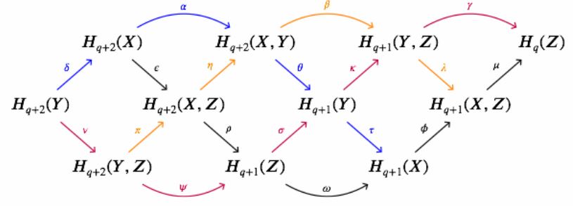
(graphics from this Maths.SE comment)

Remark

The exact sequence of a triple in prop. is what gives rise to the Cartan-Eilenberg spectral sequence for $E$-cohomology of a CW-complex $X$.

Example

For $(X,x)$ a pointed topological space and $Cone(X) = (X \wedge (I_+))/X$ its reduced cone, the long exact sequence of the triple $(\{x\}, X, Cone(X))$, prop. ,

$$0 \simeq E^q(Cone(X), \{x\}) \longrightarrow E^q(X,\{x\}) \overset{\bar \delta}{\longrightarrow} E^{q+1}(Cone(X),X) \longrightarrow E^{q+1}(Cone(X), \{x\}) \simeq 0$$

exhibits the connecting homomorphism $\bar \delta$ here as an isomorphism

$$\bar \delta \;\colon\; E^q(X,\{x\}) \overset{\simeq}{\longrightarrow} E^{q+1}(Cone(X),X) \,.$$

This is the suspension isomorphism extracted from the unreduced cohomology theory, see def. below.

Proposition

(Mayer-Vietoris sequence)

Given $E^\bullet$ an unreduced cohomology theory, def. . Given a topological space covered by the interior of two spaces as $X = Int(A) \cup Int(B)$, then for each $C \subset A \cap B$ there is a long exact sequence of cohomology groups of the form

$$\cdots \to E^{n-1}(A \cap B , C) \overset{\bar \delta}{\longrightarrow} E^n(X,C) \longrightarrow E^n(A,C) \oplus E^n(B,C) \longrightarrow E^n(A \cap B, C) \to \cdots \,.$$

e.g. (Switzer 75, theorem 7.19, Aguilar-Gitler-Prieto 02, theorem 12.1.22)

The relation

Definition

(unreduced to reduced cohomology)

Let $E^\bullet$ be an unreduced cohomology theory, def. . Define a reduced cohomology theory, def. $(\tilde E^\bullet, \sigma)$ as follows.

For $x \colon \ast \to X$ a pointed topological space, set

$$\tilde E^\bullet(X,x) \coloneqq E^\bullet(X,\{x\}) \,.$$

This is clearly functorial. Take the suspension isomorphism to be the composite

$$\sigma \;\colon\; \tilde E^{\bullet+1}(\Sigma X) = E^{\bullet+1}(\Sigma X, \{x\}) \overset{E^\bullet(p)}{\longrightarrow} E^{\bullet+1}(Cone(X),X) \overset{\bar \delta^{-1}}{\longrightarrow} E^\bullet(X,\{x\}) = \tilde E^{\bullet}(X)$$

of the isomorphism $E^\bullet(p)$ from example and the inverse of the isomorphism $\bar \delta$ from example .

Proposition

The construction in def. indeed gives a reduced cohomology theory.

(e.g. Switzer 75, 7.34)

Proof

We need to check the exactness axiom given any $A\hookrightarrow X$. By lemma we have an isomorphism

$$\tilde E^\bullet(X \cup Cone(A)) = E^\bullet(X \cup Cone(A), \{\ast\}) \overset{\simeq}{\longrightarrow} E^\bullet(X,A) \,.$$

Unwinding the constructions shows that this makes the following diagram commute:

$$\array{ \tilde E^\bullet(X\cup Cone(A)) &\overset{\simeq}{\longrightarrow}& E^\bullet(X,A) \\ \downarrow && \downarrow \\ \tilde E^\bullet(X) &=& E^\bullet(X,\{x\}) \\ \downarrow && \downarrow \\ \tilde E^\bullet(A) &=& E^\bullet(A,\{a\}) } \,,$$

where the vertical sequence on the right is exact by prop. . Hence the left vertical sequence is exact.

Definition

(reduced to unreduced cohomology)

Let $(\tilde E^\bullet, \sigma)$ be a reduced cohomology theory, def. . Define an unreduced cohomolog theory $E^\bullet$, def. , by

$$E^\bullet(X,A) \coloneqq \tilde E^\bullet( X_+ \cup Cone(A_+))$$

and let the connecting homomorphism be as in def. .

Proposition

The construction in def. indeed yields an unreduced cohomology theory.

e.g. (Switzer 75, 7.35)

Proof

Exactness holds by prop. . For excision, it is sufficient to consider the alternative formulation of lemma . For CW-inclusions, this follows immediately with lemma .

Theorem

The constructions of def. and def. constitute a pair of functors between then categories of reduced cohomology theories, def. and unreduced cohomology theories, def. which exhbit an equivalence of categories.

Proof

(…careful with checking the respect for suspension iso and connecting homomorphism..)

To see that there are natural isomorphisms relating the two composites of these two functors to the identity:

One composite is

$$\begin{aligned} E^\bullet & \mapsto (\tilde E^\bullet \colon (X,x) \mapsto E^\bullet(X,\{x\})) \\ & \mapsto ((E')^\bullet \colon (X,A) \mapsto E^\bullet( X_+ \cup Cone(A_+) ), \ast) \end{aligned} \,,$$

where on the right we have, from the construction, the reduced mapping cone of the original inclusion $A \hookrightarrow X$ with a base point adjoined. That however is isomorphic to the unreduced mapping cone of the original inclusion. With this the natural isomorphism is given by lemma .

The other composite is

$$\begin{aligned} \tilde E^\bullet & \mapsto (E^\bullet \colon (X,A) \mapsto \tilde E^\bullet(X_+ \cup Cone(A_+))) \\ & \mapsto ((\tilde E')^\bullet \colon X \mapsto \tilde E^\bullet(X_+ \cup Cone(*_+))) \end{aligned}$$

where on the right we have the reduced mapping cone of the point inclusion with a point adoined. As before, this is isomorphic to the unreduced mapping cone of the point inclusion. That finally is clearly homotopy equivalent to $X$, and so now the natural isomorphism follows with homotopy invariance.

Finally we record the following basic relation between reduced and unreduced cohomology:

Proposition

Let $E^\bullet$ be an unreduced cohomology theory, and $\tilde E^\bullet$ its reduced cohomology theory from def. . For $(X,\ast)$ a pointed topological space, then there is an identification

$$E^\bullet(X) \simeq \tilde E^\bullet(X) \oplus E^\bullet(\ast)$$

of the unreduced cohomology of $X$ with the direct sum of the reduced cohomology of $X$ and the unreduced cohomology of the base point.

Proof

The pair $\ast \hookrightarrow X$ induces the sequence

$$\cdots \to E^{\bullet-1}(\ast) \stackrel{\delta}{\longrightarrow} \tilde E^\bullet(X) \stackrel{}{\longrightarrow} E^\bullet(X) \stackrel{}{\longrightarrow} E^\bullet(\ast) \stackrel{\delta}{\longrightarrow} \tilde E^{\bullet+1}(X) \to \cdots$$

which by the exactness clause in def. is exact.

Now since the composite $\ast \to X \to \ast$ is the identity, the morphism $E^\bullet(X) \to E^\bullet(\ast)$ has a section and so is in particular an epimorphism. Therefore, by exactness, the connecting homomorphism vanishes, $\delta = 0$ and we have a short exact sequence

$$0 \to \tilde E^\bullet(X) \stackrel{}{\longrightarrow} E^\bullet(X) \stackrel{}{\longrightarrow} E^\bullet(\ast) \to 0$$

with the right map an epimorphism. Hence this is a split exact sequence and the statement follows.

Exmaple: Ordinary cohomology

(…)

References

• Wirthmuller 12, section 9

• Robert Switzer, chapter 7 (and 8-12) of Algebraic Topology - Homotopy and Homology, Die Grundlehren der Mathematischen Wissenschaften in Einzeldarstellungen, Vol. 212, Springer-Verlag, New York, N. Y., 1975.

Clutching construction and Product theorem

Idea

A quick way to construct vector bundles on n-spheres is to consider the trivial vector bundles on either hemisphere and then glue them by a bundle isomorphism on a small overlap of the two hemispheres. This is called the clutching construction. This construction may be paramneterized over some topological space $X$ to construct vector bundles on the product topological space of $X$ with an sphere. A close analysis of this parameterized clutching construction allows to prove what will be the first deep theorem about topological K-theory: the fundamental product theorem in K-theory, which characterizes the $K$-theory ring of product topological spaces $X \times S^2$ of some space $X$ with the 2-sphere as that of $X$ with one generator for the basic line bundle on the 2-sphere adjoined, subject to a relation. This is very useful for computations.

Below this theorem is used to prove the all-important Bott periodicity theorem of topological K-theory.

References

• Wirthmuller 12, p. 17 to p. 29

• Hatcher, p. 41-51

Splitting principle

Idea

The second deep fact about topological K-theory is the splitting principle which says roughly that as far as K-theory is concerned, all vector bundles essentially look like direct sums of vector bundles each of whose summands is just a line bundle. This has dramatic consequences, which we see when we discuss the Adams operations below. The proof of the splitting principle involves a careful analysis of flag spaces in vector bundles.

References

Wirthmuller 12, section 10

K-Cohomology theory

Idea

Finally we may put all the pieces together and show that the topological K-theory functor $K(-)$ indeed constitutes a generalized (Eilenberg-Steenrod) cohomology theory. In fact its ring structure makes it a multiplicative cohomology theory. Moreover, we find that the fundamental product theorem in K-theory implies a certain 2-periodicity in $K(-)$, called Bott periodicity. This makes $K$ an even periodic cohomology theory.

All these facts will be most useful for computing $K(X)$ and for using it to learn about topological spaces which is what we turn to next.

References

• Wirthmuller 12, p. 34 and previous

• Hatcher, section 2.2

• Aguilar-Gitler-Prieto 02, appendix B

Examples of K-groups

Idea

In the previous sessions we have accumulated some powerful tools for computing topological K-theory groups. Here we use these to consider examples, and compute K-theory groups for a range of interesting topological spaces. This will serve to see how topological K-theory is a finer invariant than ordinary cohomology.

References

• Chris Blair, Some K-theory examples, 2009 (pdf)

Adams operations

Idea

So far we have used that there is the operation of direct sum of vector bundles and of tensor product of vector bundles in order to exhibit the $K$-theory functor $K(-)$ as taking values in commutative rings. But in fact there are yet more operations on vector bundles. Namely instead of just taking plain tensor products, we may also form skew-symmetrized tensor products exterior products. Since these are traditionally denoted $\wedge^n(-)$, one says that $K(-)$ inherits the structure of a Lambda-ring. A clever combination of such exterior powers makes them be an abelian group homomorphism, these are the Adams operations on topological K-theory. We observe their basic properties, which make them most useful for characterizing topological spaces. As a first example we see that they immediately allow to prove something as fundamental to topology as the topological invariance of dimension.

An even more interesting application of the Adams operations is that they allow to characterite the continuous functions of Hopf invariant one. This is the next topic.

References

• Wirthmuller 12, section 11

• Hatcher, section 2.3

• Aguilar-Gitler-Prieto 02, section 10

Hopf invariant one

Idea

A crown jewel of the application of topological K-theory, is, via the Adams operations, a remarkably quick proof of a deep theorem whose original solution via another tool (the Adams spectral sequence) marks the beginning of modern homotopy theory: the Hopf invariant one problem.

A remarkable range of “exceptional” structures in mathematics is obtained by continuing the step from the real numbers to the complex numbers further to find the quaternions and then the octonions. Using the fact that all these algebras are real normed division algebras they induce fibrations between spheres: the Hopf fibrations.

These Hopf fibrations happen to take value +1 in a certain invariant, called the Hopf invariant. The Hopf invariant one theorem says that they there is in fact no other fibration with this property. In particular this implies, remarkably, that the real numbers, complex numbers, quaternions and octonions are the only real normed division algebras that exist.

References

• Hatcher, section 2.3

• Wirthmuller 12, section 12

• Marcelo Aguilar, Samuel Gitler, Carlos Prieto, section 10.6 of Algebraic topology from a homotopical viewpoint, Springer (2002) (toc pdf)

Equivariant K-theory

Idea

We saw how topological K-theory arises from pairing topology with linear algebra. There are variaous further refinements of topological K-theory obtained by refining these ingredients. In particular, if instead of plain vector spaces we start by considering vector spaces equipped with linear group actions, hence considering linear representations, then the resulting topological K-theory is what is called equivariant K-theory. This now pairs topology with representation theory. For instance this may now be evaluated on topological spaces which are themselves acted on by groups, and the resulting equivariant K-theory groups encode interesting information for instance about the fixed point loci of these group actions.

References

• Wirthmuller 12, section 14

$(\star)$ The K-theory spectrum

This section goes beyond an introduction, in that it requires more tools from algebraic topology. We include it for completeness and as outlook.

Idea

While we constructed classifying spaces originally for plain vector bundles, one finds that with just slight modification these also yield classifying space for virtual vector bundles, hence for topological K-theory. The fact that topological K-theory constitutes a generalized (Eilenberg-Steenrod) cohomology theory with long exact sequences in cohomology now implies that also these classifying spaces arrange in certain sequences. Suchsequences are called sequential spectra or just spectra, for short, and the spectrum that represents topoligcal K-theory of complex vector bundles is called KU.

The main point in its construction is the incarnation of Bott periodicity in terms of the classifying spaces. This yields an alternative proof of Bott periodicity, one that makes use of basics of the classical model structure on topological spaces.

The relevant background for this section is laid out in

• Introduction to stable homotopy theory – Classical homotopy theory

• Introduction to stable homotopy theory – Sequential Spectra

The main point is that in terms of the classifying spaces (as above)

$B U \times \mathbb{Z}$ and $U$ for $K^0$ and for $K^1$

the phenomenon of Bott periodicity (as above) is represented by the existence of weak homotopy equivalences

$$(B U) \times \mathbb{Z} \overset{\simeq_{whe}}{\longrightarrow} \Omega U$$

and

$$U \overset{\simeq_{whe}}{\longrightarrow} \Omega((B U) \times \mathbb{Z})$$

The last one is immediate, but the first one requires work, see Aguilar-Gitler-Prieto 02.

Together these show that the sequence of spaces KU with

$$KU_n \coloneqq \left\{ \array{ (B U) \times \mathbb{Z} & \vert n\;\text{even} \\ U & \vert n \; \text{odd} } \right.$$

and equipped with the above comparison maps forms a sequential spectrum which is in fact an Omega-spectrum.

Under the Brown representability theorem, this spectrum represents topological K-theory $K^\bullet(-)$ as a generalized (Eilenberg-Steenrod) cohomology theory, as above.

References

• Aguilar-Gitler-Prieto 02, appendix B.2

References

• Klaus Wirthmüller, Vector bundles and K-theory, 2012 (pdf)

• Allen Hatcher, Vector bundles and K-theory (web)

• Marcelo Aguilar, Samuel Gitler, Carlos Prieto, Algebraic topology from a homotopical viewpoint, Springer (2002) (toc pdf)