nLab cohomotopy
Context
Homotopy theory
homotopy theory, (∞,1)-category theory, homotopy type theory
flavors: stable, equivariant, rational, p-adic, proper, geometric, cohesive, directed…
models: topological, simplicial, localic, …
see also algebraic topology
Introductions
Definitions
Paths and cylinders
Homotopy groups
Basic facts
Theorems
Cohomology
Special and general types
-
group cohomology, nonabelian group cohomology, Lie group cohomology
-
-
cohomology with constant coefficients / with a local system of coefficients
Special notions
Variants
-
differential cohomology
Extra structure
Operations
Theorems
Manifolds and cobordisms
manifolds and cobordisms
cobordism theory, Introduction
Definitions
Genera and invariants
Classification
Theorems
Spheres
Contents
- Idea
- Properties
- Hopf degree theorem
- Poincaré–Hopf theorem
- Relation to Freudenthal suspension theorem
- Smooth representatives
- Reduced Cohomotopy
- Pontryagin isomorphism between Cohomotopy and framed Cobordism
- Composition/product in Cohomotopy
- Cohomotopy charge map and Relation to configuration spaces
- Complex-rational Cohomotopy and moduli space of Yang-Mills monopoles
- Examples
- Related concepts
- References
Idea
General
Cohomotopy cohomology theory is the (non-abelian) generalized cohomology theory whose cocycle spaces are spaces of maps into an n-sphere, hence whose cohomology classes are homotopy classes of maps into an n-sphere:
So, dually to how homotopy groups
are groups of homotopy classes of maps out of spheres, Cohomotopy sets are sets of homotopy classes of maps into spheres, whence the dual name.
If instead one considers only the stable aspect of Cohomotopy sets, by mapping into the stabilization of the spheres, hence into (some suspension of) the sphere spectrum, then one speaks of stable Cohomotopy, written
In other words, the generalized (Eilenberg-Steenrod) cohomology theory which is represented by the sphere spectrum is stable Cohomotopy.
Remark
(terminology)
Therefore “Cohomotopy theory” is really shorthand for “Cohomotopy cohomology theory” and as such is dual to homotopy homology theory, which in the stable case is known as stable homotopy homology theory.
In particular, cohomotopy theory is a concrete particular and not dual to the abstract general of homotopy theory; and is hence also not on par with the abstract general of cohomology theory. Rather, Cohomotopy theory is one instance of a cohomology theory, and as such is a sibling of ordinary cohomology theory (HR-theory)), K-theory, etc.
To emphasize this, one might, in the stable case, say -theory instead of “stable Cohomotopy theory”; where denotes the sphere spectrum. In the unstable case there is no widely adopted notation, but one might consider saying “-theory” (with the established symbol for (co)homotopy groups) or -theory (with “” for n-spheres ) for unstable Cohomotopy theory.
In any case, to highlight that Cohomotopy theory is a concrete particular and not an abstract general, it makes good sense to capitalize the term and speak of Cohomotopy cohomology theory or just Cohomotopy theory, for short.
The following table indicates the pattern:
As for any generalized cohomology theory there are immediate variants to plain Cohomotopy theory, as shown in the following table:
| flavours of Cohomotopy cohomology theory | cohomology (full or rational) | equivariant cohomology (full or rational) |
|---|---|---|
| non-abelian cohomology | Cohomotopy (full or rational) | equivariant Cohomotopy |
| twisted cohomology (full or rational) | twisted Cohomotopy | twisted equivariant Cohomotopy |
| stable cohomology (full or rational) | stable Cohomotopy | equivariant stable Cohomotopy |
| differential cohomology | differential Cohomotopy | equivariant differential cohomotopy |
| persistent cohomology | persistent Cohomotopy | persistent equivariant Cohomotopy |
As the absolute cohomology theory
In some sense Cohomotopy is the most fundamental of all generalized cohomology theories (“The Music of the Spheres”).
Concretely, stable Cohomotopy cohomology theory is the initial object among multiplicative cohomology theories, in that the sphere spectrum is the initial object in (E-infinity) ring spectra. This means that for any other multiplicative cohomology theory there is an essentially unique multiplicative natural transformation
from Cohomotopy cohomology groups to -cohomology groups – the Boardman homomorphism.
Specifically for the algebraic K-theory of a field (such as a prime field ) there is such a comparison morphism; and another way how stable Cohomotopy is the most fundamental of all K-theories is that it is equivalently the algebraic K-theory over the “absolute base”, namely over the “field with one element” (see there for more):
For example, for KU and in the case of -equivariant cohomology theory (equivariant Cohomotopy theory and equivariant K-theory) the Boardman homomorphism (1) gives the comparison map
from the Burnside ring to the representation ring of the finite group , by forming permutation representations; where we may think of the Burnside ring as being the representation ring over the “field with one element” (see e.g. Chu-Lorscheid-Santhanam 10), as indicated above.
So far, this applies to stable Cohomotopy theory, which historically has received almost all the attention. But, while stabilization makes the immensely rich nature of homotopy theory a tad more tractable, it is only an approximation (just the first Goodwillie derivative!) of full unstable/non-abelian cohomology. Hence the one concept more fundamental than stable Cohomotopy theory is actual Cohomotopy theory.
For example, the classification of Yang-Mills instantons on is typically regarded in the non-abelian cohomology theory represented by the classifying space of the special unitary group (for , starting with SU(2))
But since the one-point compactification of 4d Euclidean space is the 4-sphere , this classification factors through one in unstable Cohomotopy theory, via the “unstable Boardman homomorphism” representing the generator of the 4th homotopy group of (see there)
(see SS 19, p. 9-10) This is the tip of an iceberg. Which needs to be discussed elsewhere.
Properties
Hopf degree theorem
Proposition
Let be a natural number and be a connected orientable closed manifold of dimension . Then the th cohomotopy classes of are in bijection to the degree of the representing functions, hence the canonical function
from th cohomotopy to th integral cohomology is a bijection.
(e.g. Kosinski 93, IX (5.8))
Poincaré–Hopf theorem
Relation to Freudenthal suspension theorem
relation to the Freudenthal suspension theorem (Spanier 49, section 9)
Smooth representatives
For a compact smooth manifold, there is a smooth function representing every cohomotopy class (with respect to the standard smooth structure on the sphere manifold).
Reduced Cohomotopy
For some purposes (such as in stating Pontryagin's theorem below) it is more natural to use reduced Cohomotopy:
For a pointed homotopy type/cofibrant pointed topological space, its reduced -Cohomotopy is the set of connected components in the mapping space of pointed functions to the n-sphere (for any choice of basepoint on the latter, then naturally thought of as ):
However, the difference between reduced and unreduced Cohomotopy is small:
Proposition
For a positive natural number and a pointed topological space/pointed homotopy type, the canonical morphism from reduced (2) to unreduced Cohomotopy of in degree is an isomorphism:
Proof
Observe that
(where is the evaluation map at ) is a homotopy fiber sequence as soon as is represented by a cell complex (e.g. CW-complex). This follows either from the pullback-power axiom in the classical model structure on topological spaces, or, more abstractly from the characterization of derived hom-spaces in coslice (infinity,1)-categories here.
Therefore we have the corresponding long exact sequence of homotopy groups, which starts out as
By exactness, this yields the claim for ; while for it gives the desired isomorphism only up to a possibly non-trivial quotient by an action of :
Hence it is now sufficient to see that the -action on reduced 1-Cohomotopy is always trivial:
Now, the action of takes to any such that in , with . But using the group-structure on we have that one such is given by , which yields and hence .
Pontryagin isomorphism between Cohomotopy and framed Cobordism
Pontryagin's theorem (Pontryagin 38, Pontryagin 55) is an identification of cobordism classes of normally framed submanifolds of codimension in a closed manifold with the -Cohomotopy of that manifold – the homotopy classes of maps into the n-sphere, which is exhibited by the Cohomotopy charge map, often known as the Pontryagin-Thom collapse construction:
The analogous statement identifying cobordism classes of normally oriented submanifolds with homotopy classes of maps into the universal special orthogonal Thom space is Thom's theorem (Thom 54). Both statements, as well as their joint generalization to other tangential structures and notably their stabilization to Whitehead-generalized Cobordism cohomology theory, have come to be widely known as the Pontryagin-Thom collapse construction, or similar, and form the basis of modern cobordism theory and its application in stable homotopy theory.
For a closed smooth manifold of dimension , the assignment of Cohomotopy charge (the Pontryagin-Thom construction, in this unstable and framed version due to Pontrjagin 55, see review in Kosinski 93, IX.5, Milnor 97) identifies the set
of cobordism classes of closed and normally framed submanifolds of dimension inside with the cohomotopy of in degree
(e.g. Kosinski 93, IX Theorem (5.5))
In particular, by this bijection the canonical group structure on cobordism groups in sufficiently high codimension (essentially given by disjoint union of submanifolds) this way induces a group structure on the cohomotopy sets in sufficiently high degree.
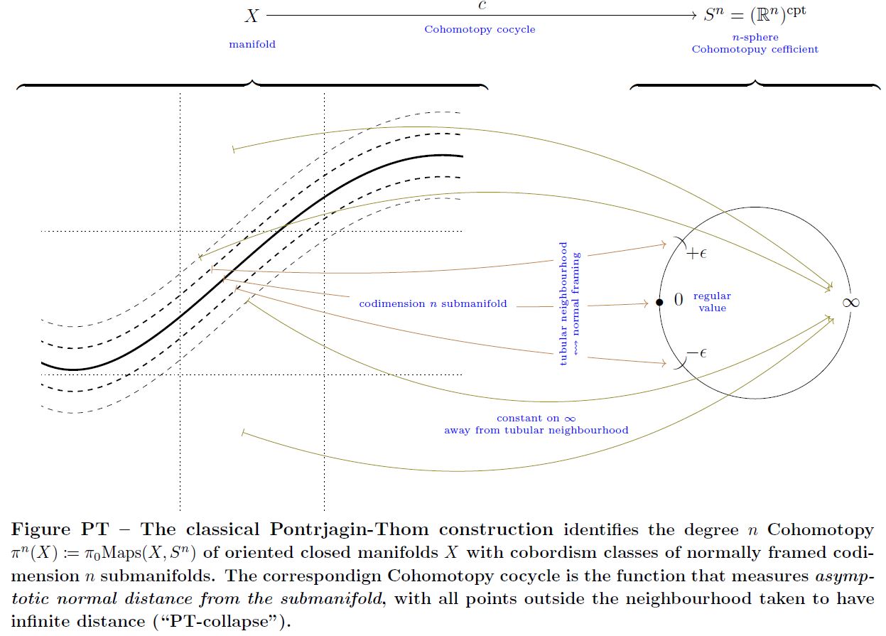
graphics grabbed form Sati-Schreiber 19
Here the normal framing of the submanifolds plays the role of the charge in Cohomotopy which they carry:
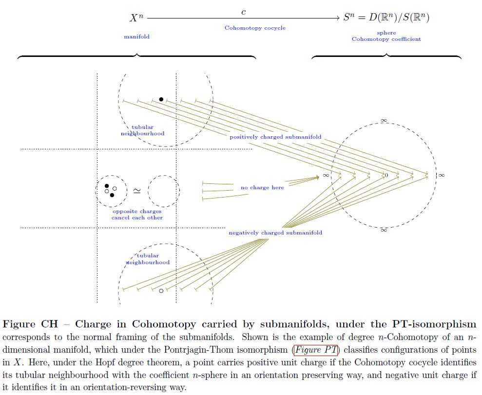
graphics grabbed form Sati-Schreiber 19
For example:
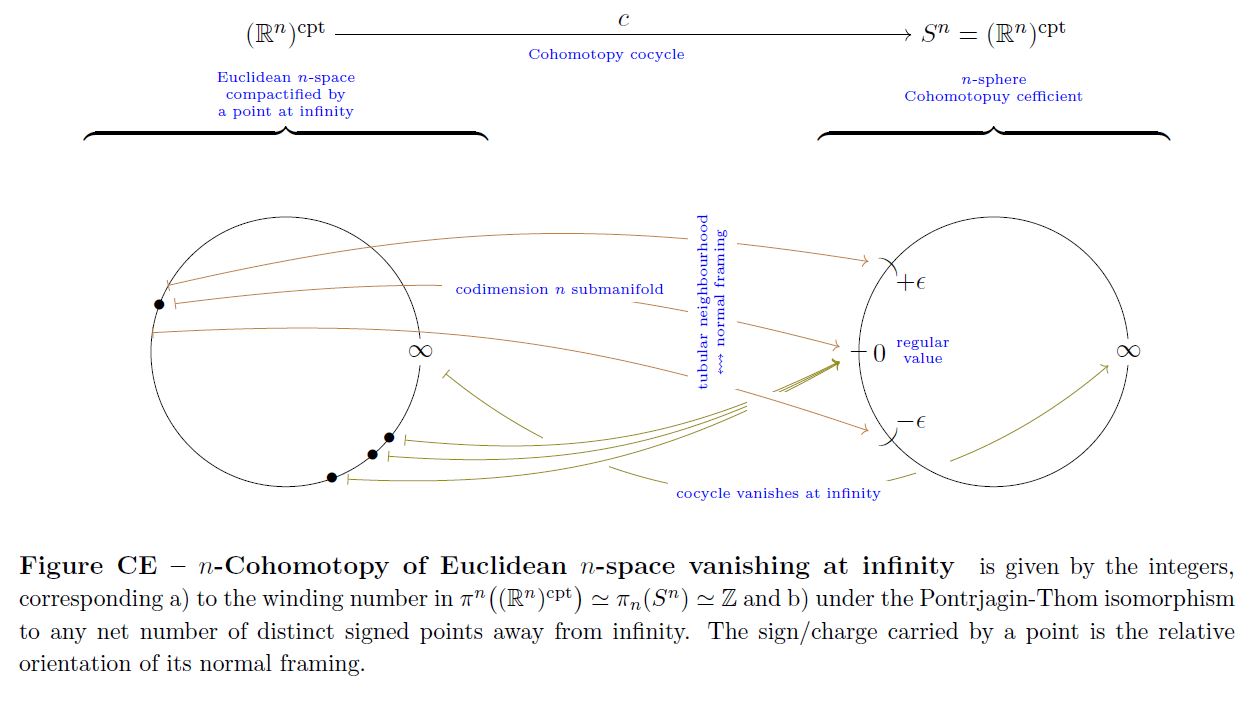
graphics grabbed form Sati-Schreiber 19
This construction generalizes to equivariant cohomotopy, see there.
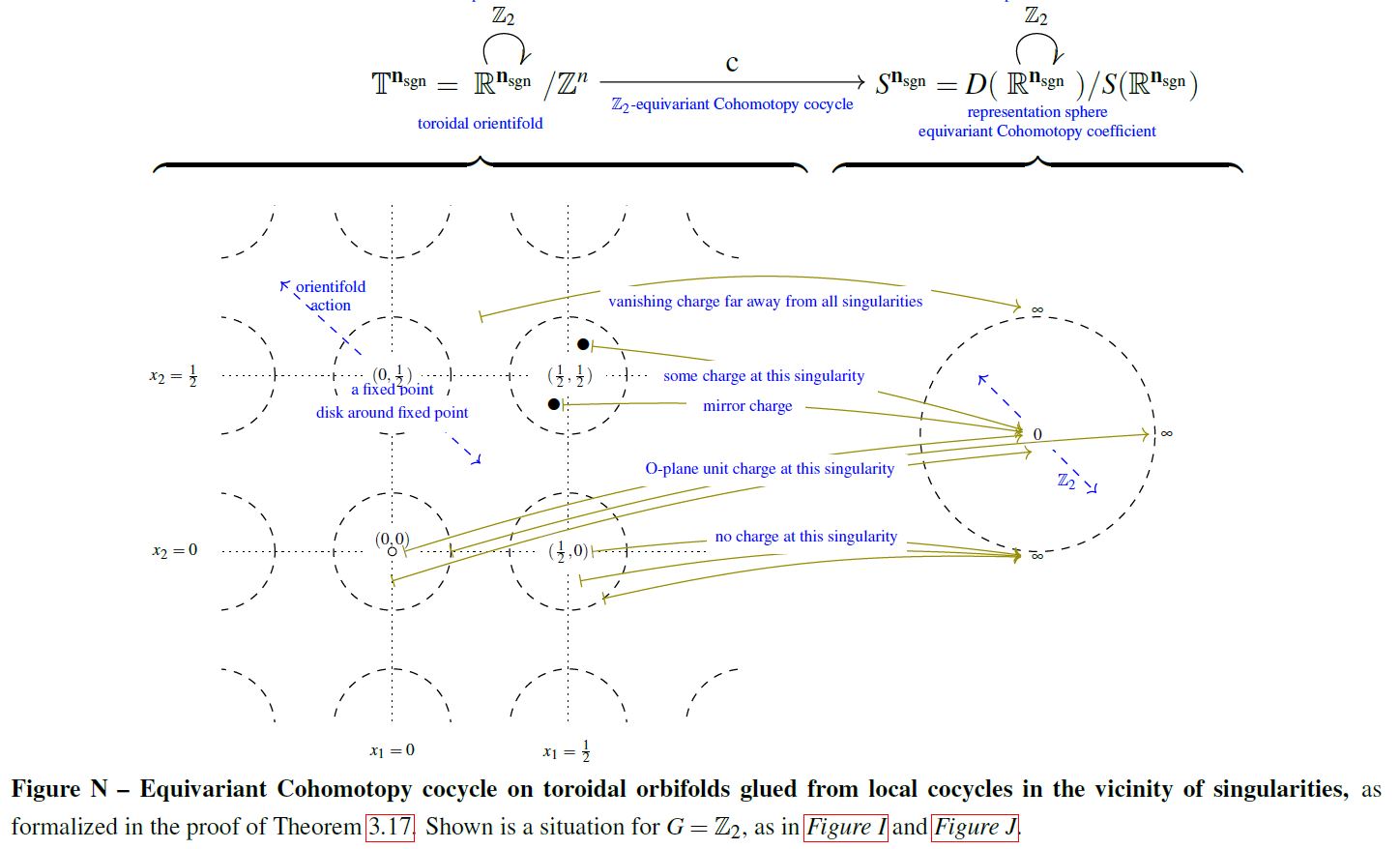
With the equivariant Hopf degree theorem the above example has the following -equivariant version (see there):
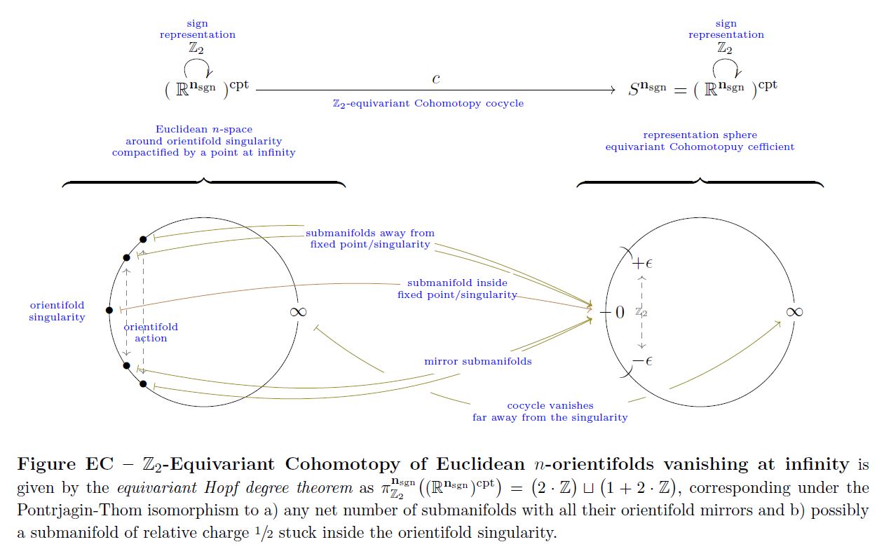
graphics grabbed form Sati-Schreiber 19
Further by the equivariant Hopf degree theorem (see there), this example generalizes to equivariant cohomotopy of toroidal orientifolds:
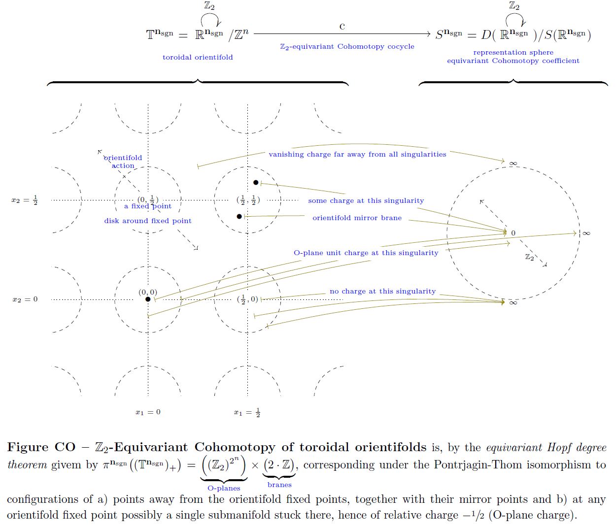
graphics grabbed form Sati-Schreiber 19
Composition/product in Cohomotopy
Under the Pontryagin-Thom isomorphism (above) the product in Cohomotopy, i.e. the composition operation
corresponds to forming product manifolds of submanifolds, in that (see also Kosinski 93, Section IX 6.1):
This is exhibited by the following pasting diagram of pullbacks/fiber products (repeatedly using the pasting law):
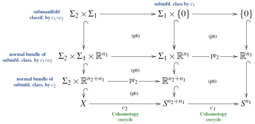
Here the vertical inclusions are the defining ones of the submanifolds or of their normal bundles, identified with some choice of tubular neighbourhoods.
Cohomotopy charge map and Relation to configuration spaces
The Cohomotopy charge map is the function that assigns to a configuration of points their total charge as measured in Cohomotopy-cohomology theory.
This is alternatively known as the “electric field map” (Salvatore 01 following Segal 73, Section 1, see also Knudsen 18, p. 49) or the “scanning map” (Kallel 98).
For the Cohomotopy charge map is the continuous function
from the configuration space of points in the Euclidean space to the -Cohomotopy cocycle space vanishing at infinity on the Euclidean space(which is equivalently the space of pointed maps from the one-point compactification to itself, and hence equivalently the -fold iterated based loop space of the D-sphere), which sends a configuration of points in , each regarded as carrying unit charge to their total charge as measured in Cohomotopy-cohomology theory (Segal 73, Section 3).
This has evident generalizations to other manifolds than just Euclidean spaces, to spaces of labeleed configurations and to equivariant Cohomotopy. The following graphics illustrates the Cohomotopy charge map on G-space tori for with values in -equivariant Cohomotopy:
graphics grabbed from SS 19
In some situations the Cohomotopy charge map is a weak homotopy equivalence and hence exhibits, for all purposes of homotopy theory, the Cohomotopy cocycle space of Cohomotopy charges as an equivalent reflection of the configuration space of points.
Proposition
(group completion on configuration space of points is iterated based loop space)
from the full unordered and unlabeled configuration space (here) of Euclidean space to the -fold iterated based loop space of the D-sphere, exhibits the group completion (here) of the configuration space monoid
Proposition
(Cohomotopy charge map is weak homotopy equivalence on sphere-labeled configuration space of points)
For with , the Cohomotopy charge map (3)
is a weak homotopy equivalence from the configuration space (here) of unordered points with labels in and vanishing at the base point of the label space to the -fold iterated loop space of the D+k-sphere.
The May-Segal theorem generalizes from Euclidean space to closed smooth manifolds if at the same time one passes from plain Cohomotopy to twisted Cohomotopy, twisted, via the J-homomorphism, by the tangent bundle:
Proposition
Let
-
be a smooth closed manifold of dimension ;
Then the Cohomotopy charge map constitutes a weak homotopy equivalence
between
-
the J-twisted (n+k)-Cohomotopy space of , hence the space of sections of the -spherical fibration over which is associated via the tangent bundle by the O(n)-action on
-
the configuration space of points on with labels in .
(Bödigheimer 87, Prop. 2, following McDuff 75)
Remark
In the special case that the closed manifold in Prop. is parallelizable, hence that its tangent bundle is trivializable, the statement of Prop. reduces to this:
Let
-
be a parallelizable closed manifold of dimension ;
Then the Cohomotopy charge map constitutes a weak homotopy equivalence
between
-
-Cohomotopy space of , hence the space of maps from to the (n+k)-sphere
-
the configuration space of points on with labels in .
Complex-rational Cohomotopy and moduli space of Yang-Mills monopoles
The assignment of scattering amplitudes of monopoles in SU(2)-Yang-Mills theory is a diffeomorphism
identifying the moduli space of monopoles of number with the space of complex-rational functions form the Riemann sphere to itself, of degree (hence the cocycle space of complex-rational 2-Cohomotopy).
(Atiyah-Hitchin 88, Theorem 2.10)
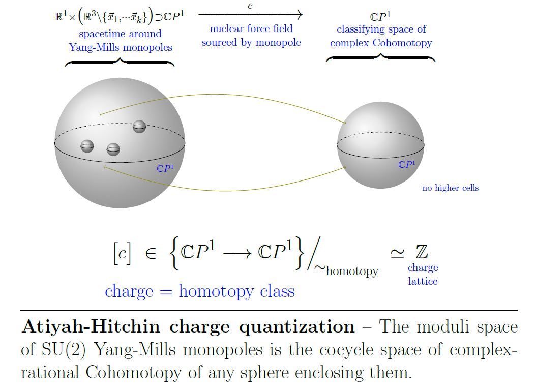
This is a non-abelian analog of the Dirac charge quantization of the electromagnetic field, with ordinary cohomology replaced by Cohomotopy cohomology theory.
Examples
Cohomotopy in the lowest dimensions
Since the 0-sphere is the disjoint union of two points, -cohomotopy corresponds to the powerset of the connected components of a space.
Further, the -sphere is understood as the empty space. Since the only map to the empty space is the identity map from the empty space, the -cohomotopy of a space is measuring whether that space is empty. In the context of homotopy type theory, this is the same as negation.
Of projective spaces
Cohomotopy sets of projective spaces are computed in West 71
Of 4-Manifolds
Let be a 4-manifold which is connected and oriented.
The Pontryagin-Thom construction as above gives for the commuting diagram of sets
where denotes cohomotopy sets, denotes ordinary cohomology, denotes ordinary homology and is normally framed cobordism classes of normally framed submanifolds. Finally is the operation of pullback of the generating integral cohomology class on (by the nature of Eilenberg-MacLane spaces):
Now
-
, , are isomorphisms
-
is an isomorphism if is “odd” in that it contains at least one closed oriented surface of odd self-intersection, otherwise becomes an isomorphism on a -quotient group of (which is a group via the group-structure of the 3-sphere (SU(2)))
Related concepts
| flavours of Cohomotopy cohomology theory | cohomology (full or rational) | equivariant cohomology (full or rational) |
|---|---|---|
| non-abelian cohomology | Cohomotopy (full or rational) | equivariant Cohomotopy |
| twisted cohomology (full or rational) | twisted Cohomotopy | twisted equivariant Cohomotopy |
| stable cohomology (full or rational) | stable Cohomotopy | equivariant stable Cohomotopy |
| differential cohomology | differential Cohomotopy | equivariant differential cohomotopy |
| persistent cohomology | persistent Cohomotopy | persistent equivariant Cohomotopy |
References
General
Original articles:
-
Karol Borsuk, Sur les groupes des classes de transformations continues, CR Acad. Sci. Paris 202 1400-1403 (1936) 2-3
-
Lev Pontrjagin, Classification of continuous maps of a complex into a sphere, Communication I, Doklady Akademii Nauk SSSR 19(3) (1938), 147-149
-
Edwin Spanier, Borsuk’s Cohomotopy Groups, Annals of Mathematics Second Series, Vol. 50, No. 1 (Jan., 1949), pp. 203-245 (jstor:1969362)
-
Franklin Peterson, Some Results on Cohomotopy Groups, American Journal of Mathematics Vol. 78, No. 2 (Apr., 1956), pp. 243-258 (jstor:2372514)
-
Jan Jaworowski, Generalized cohomotopy groups as limit groups, Fundamenta Mathematicae 50 (1962), 393-402 (doi:10.4064/fm-50-4-333-340, pdf)
See also
-
Wikipedia, Cohomotopy group
Further discussion:
- Laurence Taylor, The principal fibration sequence and the second cohomotopy set, Proceedings of the Freedman Fest, 235251, Geom. Topol. Monogr., 18, Coventry, 2012 (arXiv:0910.1781, doi:10.2140/gtm.2012.18.235)
On (stable) motivic Cohomotopy of schemes (as motivic homotopy classes of maps into motivic Tate spheres):
-
Aravind Asok, Jean Fasel, Mrinal Kanti Das, Euler class groups and motivic stable cohomotopy, Journal of the EMS 24 8 (2022) 2775–2822 [arXiv:1601.05723, doi:10.4171/jems/1156]
-
Samuel Lerbet, Motivic stable cohomotopy and unimodular rows, Advances in Mathematics 436 109415 (2024) [arXiv:2206.11688, doi:10.1016/j.aim.2023.109415]
Pontrjagin-Thom construction
Pontrjagin’s construction
General
The Pontryagin theorem, i.e. the unstable and framed version of the Pontrjagin-Thom construction, identifying cobordism classes of normally framed submanifolds with their Cohomotopy charge in unstable Borsuk-Spanier Cohomotopy sets, is due to:
-
Lev Pontrjagin, Classification of continuous maps of a complex into a sphere, Communication I, Doklady Akademii Nauk SSSR 19(3) (1938), 147-149
-
Lev Pontryagin, Homotopy classification of mappings of an (n+2)-dimensional sphere on an n-dimensional one, Doklady Akad. Nauk SSSR (N.S.) 19 (1950), 957–959 (pdf)
(both available in English translation in Gamkrelidze 86),
as presented more comprehensively in:
- Lev Pontrjagin, Smooth manifolds and their applications in Homotopy theory, Trudy Mat. Inst. im Steklov, No 45, Izdat. Akad. Nauk. USSR, Moscow, 1955 (AMS Translation Series 2, Vol. 11, 1959) (doi:10.1142/9789812772107_0001, pdf)
The Pontrjagin theorem must have been known to Pontrjagin at least by 1936, when he announced the computation of the second stem of homotopy groups of spheres:
- Lev Pontrjagin, Sur les transformations des sphères en sphères (pdf) in: Comptes Rendus du Congrès International des Mathématiques – Oslo 1936 (pdf)
Review:
-
Daniel Freed, Karen Uhlenbeck, Appendix B of: Instantons and Four-Manifolds, Mathematical Sciences Research Institute Publications, Springer 1991 (doi:10.1007/978-1-4613-9703-8)
-
Antoni Kosinski, chapter IX of: Differential manifolds, Academic Press (1993) [pdf, ISBN:978-0-12-421850-5]
-
John Milnor, Chapter 7 of: Topology from the differentiable viewpoint, Princeton University Press, 1997. (ISBN:9780691048338, pdf)
-
Mladen Bestvina (notes by Adam Keenan), Chapter 16 in: Differentiable Topology and Geometry, 2002 (pdf)
-
Michel Kervaire, La méthode de Pontryagin pour la classification des applications sur une sphère, in: E. Vesentini (ed.), Topologia Differenziale, CIME Summer Schools, vol. 26, Springer 2011 (doi:10.1007/978-3-642-10988-1_3)
-
Rustam Sadykov, Section 1 of: Elements of Surgery Theory, 2013 (pdf, pdf)
-
András Csépai, Stable Pontryagin-Thom construction for proper maps, Period Math Hung 80, 259–268 (2020) (arXiv:1905.07734, doi:10.1007/s10998-020-00327-0)
Discussion of the early history:
Twisted/equivariant generalizations
The (fairly straightforward) generalization of the Pontrjagin theorem to the twisted Pontrjagin theorem, identifying twisted Cohomotopy with cobordism classes of normally twisted-framed submanifolds, is made explicit in:
- James Cruickshank, Lemma 5.2 using Sec. 5.1 in: Twisted homotopy theory and the geometric equivariant 1-stem, Topology and its Applications Volume 129, Issue 3, 1 April 2003, Pages 251-271 (doi:10.1016/S0166-8641(02)00183-9)
A general equivariant Pontrjagin theorem – relating equivariant Cohomotopy to normal equivariant framed submanifolds – remains elusive, but on free G-manifolds it is again straightforward (and reduces to the twisted Pontrjagin theorem on the quotient space), made explicit in:
- James Cruickshank, Thm. 5.0.6, Cor. 6.0.13 in: Twisted Cobordism and its Relationship to Equivariant Homotopy Theory, 1999 (pdf, pdf)
In negative codimension
In negative codimension, the Cohomotopy charge map from the Pontrjagin theorem gives the May-Segal theorem, now identifying Cohomotopy cocycle spaces with configuration spaces of points:
-
Peter May, The geometry of iterated loop spaces, Springer 1972 (pdf)
-
Graeme Segal, Configuration-spaces and iterated loop-spaces, Invent. Math. 21 (1973), 213–221. MR 0331377 (pdf)
c Generalization of these constructions and results is due to
-
Dusa McDuff, Configuration spaces of positive and negative particles, Topology Volume 14, Issue 1, March 1975, Pages 91-107 (doi:10.1016/0040-9383(75)90038-5)
-
Carl-Friedrich Bödigheimer, Stable splittings of mapping spaces, Algebraic topology. Springer 1987. 174-187 (pdf, pdf)
Thom’s construction
Thom's theorem i.e. the unstable and oriented version of the Pontrjagin-Thom construction, identifying cobordism classes of normally oriented submanifolds with homotopy classes of maps to the universal special orthogonal Thom space , is due to:
- René Thom, Quelques propriétés globales des variétés différentiables, Comment. Math. Helv. 28, (1954). 17-86 (doi:10.1007/BF02566923, dml:139072, digiz:GDZPPN002056259, pdf)
Textbook accounts:
- Robert Stong, Notes on Cobordism theory, 1968 (toc pdf, publisher page)
Lashof’s construction
The joint generalization of Pontryagin 38a, 55 (framing structure) and Thom 54 (orientation structure) to any family of tangential structures (“(B,f)-structure”) is first made explicit in
- Richard Lashof, Poincaré duality and cobordism, Trans. AMS 109 (1963), 257-277 (doi:10.1090/S0002-9947-1963-0156357-4)
and the general statement that has come to be known as the Pontryagin-Thom isomorphism (identifying the stable cobordism classes of normally (B,f)-structured submanifolds with homotopy classes of maps to the Thom spectrum Mf) is really due to Lashof 63, Theorem C.
Textbook accounts:
-
Theodor Bröcker, Tammo tom Dieck, Satz 3.1 & 4.9 in: Kobordismentheorie, Lecture Notes in Mathematics 178, Springer (1970) [ISBN:9783540053415]
-
Stanley Kochman, section 1.5 of: Bordism, Stable Homotopy and Adams Spectral Sequences, AMS 1996
-
Yuli Rudyak, On Thom spectra, Orientability and Cobordism, Springer 1998 (pdf)
Lecture notes:
-
John Francis, Topology of manifolds course notes (2010) (web), Lecture 3: Thom’s theorem (pdf), Lecture 4 Transversality (notes by I. Bobkova) (pdf)
-
Cary Malkiewich, Section 3 of: Unoriented cobordism and , 2011 (pdf)
-
Tom Weston, Part I of An introduction to cobordism theory (pdf)
See also:
Examples
Cohomotopy sets of projective spaces:
- Robert West, Some Cohomotopy of Projective Space, Indiana University Mathematics Journal Vol. 20, No. 9 (March, 1971), pp. 807-827 (jstor:24890146)
Cohomotopy sets of 4-manifolds:
-
Nobuo Shimada, Homotopy classification of mappings of a 4-dimensional complex into a 2-dimensional sphere, Nagoya Math. J., Volume 5 (1953), 127-144 (euclid:nmj/1118799399)
-
Daniel Freed, Karen Uhlenbeck, Appendix B of: Instantons and Four-Manifolds, Mathematical Sciences Research Institute Publications, Springer 1991 (doi:10.1007/978-1-4613-9703-8)
-
Robion Kirby, Paul Melvin, Peter Teichner, Cohomotopy sets of 4-manifolds, Geometry & Topology Monographs 18 (2012) 161–190 (arXiv:1203.1608, doi:10.2140/gtm.2012.18.161)
Cohomotopy sets of Thom spaces:
- Thomas Rot, Homotopy classes of proper maps out of vector bundles, Arch. Math. 114, 107–117 (2020 (arXiv:1808.08073, doi:10.1007/s00013-019-01372-z)
In relation to quaternionic line bundles over 5-manifolds:
- Panagiotis Konstantis, Vector bundles and cohomotopies of spin 5-manifolds, Homology, Homotopy and Applications Volume 23 (2021) Number 1 (arXiv:1812.06547, doi:10.4310/HHA.2021.v23.n1.a9)
Cohomotopy sets of spin-manifolds in co-degree 1:
- Panagiotis Konstantis, A counting invariant for maps into spheres and for zero loci of sections of vector bundles, Abh. Math. Semin. Univ. Hambg. (2020) (arXiv:1911.03214, doi:10.1007/s12188-020-00228-6)
Cohomotopy cocycle spaces
Discussion of Cohomotopy cocycle spaces (i.e. spaces of maps into an n-sphere):
-
Vagn Lundsgaard Hansen, The homotopy problem for the components in the space of maps on the -sphere, Quart. J. Math. Oxford Ser. (3) 25 (1974), 313-321 (DOI:10.1093/qmath/25.1.313)
-
Vagn Lundsgaard Hansen, On Spaces of Maps of -Manifolds Into the -Sphere, Transactions of the American Mathematical Society, Vol. 265, No. 1 (May, 1981), pp. 273-281 (jstor:1998494)
-
Victor Vassiliev, Twisted homology of configuration spaces, homology of spaces of equivariant maps, and stable homology of spaces of non-resultant systems of real homogeneous polynomials (arXiv:1809.05632)
-
Douglas Ravenel, What we still don’t know about loop spaces of spheres, in: Mark Mahowald, Stewart Priddy (eds.), Homotopy Theory via Algebraic Geometry and Group Representations, Contemporary Mathematics 220, AMS 1998 (pdf, pdf, doi:10.1090/conm/220)
Discussion of cocycle spaces for rational Cohomotopy (see also at rational model of mapping spaces):
- Jesper Møller, Martin Raussen, Rational Homotopy of Spaces of Maps Into Spheres and Complex Projective Spaces, Transactions of the American Mathematical Society Vol. 292, No. 2 (Dec., 1985), pp. 721-732 (jstor:2000242)
Relation to knots and links
- Maths.SE, Framed Cobordism Classes of links in
In computational topology
Discussion of Cohomotopy-sets in computational topology:
-
Martin Čadek, Marek Krčál, Jiří Matoušek, Francis Sergeraert, Lukáš Vokřínek, Uli Wagner, Computing all maps into a sphere, Journal of the ACM, Volume 61 Issue 3, May 2014 Article No. 1 (arxiv:1105.6257)
-
Lukáš Vokřínek, Decidability of the extension problem for maps into odd-dimensional spheres, Discrete Comput Geom (2017) 57: 1 (arXiv:1401.3758)
Cohomotopy in topological data analysis
Introducing persistent cohomotopy as a tool in topological data analysis, improving on the use of well groups from persistent homology:
-
Peter Franek, Marek Krčál, On Computability and Triviality of Well Groups, Discrete Comput Geom 56 (2016) 126 (arXiv:1501.03641, doi:10.1007/s00454-016-9794-2)
-
Peter Franek, Marek Krčál, Persistence of Zero Sets, Homology, Homotopy and Applications, 19 2 (2017) (arXiv:1507.04310, doi:10.4310/HHA.2017.v19.n2.a16)
-
Peter Franek, Marek Krčál, Hubert Wagner, Solving equations and optimization problems with uncertainty, J Appl. and Comput. Topology 1 (2018) 297 (arxiv:1607.06344, doi:10.1007/s41468-017-0009-6)
Review:
-
Peter Franek, Marek Krčál, Cohomotopy groups capture robust Properties of Zero Sets via Homotopy Theory, talk at ACAT meeting 2015 pdf
-
Urs Schreiber on joint work with Hisham Sati: New Foundations for TDA – Cohomotopy, (May 2022)
Equivariant Cohomotopy
Discussion of the stable cohomotopy (framed cobordism cohomology theory) in the equivariant cohomology-version of cohomotopy (equivariant cohomotopy):
-
Arthur Wasserman, section 3 of Equivariant differential topology, Topology Vol. 8, pp. 127-150, 1969 (pdf)
-
James Cruickshank, Twisted homotopy theory and the geometric equivariant 1-stem, Topology and its Applications Volume 129, Issue 3, 1 April 2003, Pages 251-271 (arXiv:10.1016/S0166-8641(02)00183-9)
and in the twisted cohomology-version (twisted cohomotopy)
- James Cruickshank, Section 7 of Twisted homotopy theory and the geometric equivariant 1-stem, Topology and its Applications Volume 129, Issue 3, 1 April 2003, Pages 251-271 (arXiv:10.1016/S0166-8641(02)00183-9)
Discussion of M-brane physics in terms of rational equivariant cohomotopy:
- John Huerta, Hisham Sati, Urs Schreiber, Real ADE-equivariant (co)homotopy and Super M-branes (arXiv:1805.05987)
and in terms of twisted cohomotopy:
-
Domenico Fiorenza, Hisham Sati, Urs Schreiber, Section 3 of Twisted Cohomotopy implies M-theory anomaly cancellation (arXiv:1904.10207)
-
Domenico Fiorenza, Hisham Sati, Urs Schreiber, Twisted Cohomotopy implies level quantization of the full 6d Wess-Zumino-term of the M5-brane (arXiv:1906.07417)
-
Hisham Sati, Urs Schreiber, Equivariant Cohomotopy implies orientifold tadpole cancellation (arXiv:1909.12277)
In spectral geometry
Discussion of smooth functions into the 4-sphere in the context of Connes-Lott models in spectral non-commutative geometry:
-
Ali Chamseddine, Alain Connes, Viatcheslav Mukhanov, Quanta of Geometry: Noncommutative Aspects, Phys. Rev. Lett. 114 (2015) 9, 091302 (arXiv:1409.2471)
-
Ali Chamseddine, Alain Connes, Viatcheslav Mukhanov, Geometry and the Quantum: Basics, JHEP 12 (2014) 098 (arXiv:1411.0977)
-
Alain Connes, section 4 of Geometry and the Quantum, in Foundations of Mathematics and Physics One Century After Hilbert, Springer 2018. 159-196 (arXiv:1703.02470, doi:10.1007/978-3-319-64813-2)
Last revised on March 4, 2024 at 23:42:51. See the history of this page for a list of all contributions to it.