nLab Planck's constant
Context
Physics
physics, mathematical physics, philosophy of physics
Surveys, textbooks and lecture notes
theory (physics), model (physics)
experiment, measurement, computable physics
-
-
-
Axiomatizations
-
Tools
-
Structural phenomena
-
Types of quantum field thories
-
Contents
Idea
What is called Planck’s constant in physics and specifically in quantum physics (after Max Planck) is a physical unit of “action” which sets the scale at which effects of quantum physics are genuinely important and physics is no longer well approximated by classical mechanics/classical field theory.
This is discussed in the section:
In the mathematical formulation of the theory, Planck’s constant is the choice of unit in the short exact sequence which governs the prequantization lift from real (differential) cohomology to (differential) integral cohomology. The integrality of here is the very “quantum”-ness of quantum theory, and this is what Planck’s constant parameterizes. This is discussed in the section:
Finally, when infinitesimally approximating this quantization step in perturbation theory in (see at formal deformation quantization), then Planck’s constant is the very formal expansion parameter of the deformation. This is discussed in the section:
Applied to the key example of perturbative quantum field theory it turns out that the powers of in contributions to the Feynman perturbation series essentially correspond to the loop order of the given Feynman diagram. This is discussed in the section
As a physical constant
The original Planck constant is a quantum of action. It may be illustrated in the case of the electromagnetic field by the fact that each of its quanta – a photon – carries an energy that is fixed by its frequency (cycles per second) according to the relation . Thus, the energy emitted by a laser beam of fixed frequency is an integer multiple of a packet of energy , where is the number of photons emitted.
As a fundamental physical constant, has dimension . In meter-kilogram-second (MKS) units, its value is exactly
by the SI definition of the kilogram.
The reduced Planck constant or Dirac constant [Dirac 1933 p. 208]
is the proportionality constant that relates energy (of a photon) to angular frequency (radians per second as opposed to cycles per second), so that .
In geometric quantization
Basic definition
The step of prequantization is about refining data in (differential) real cohomology to (differential) integral cohomology. Often this is understood in terms of the canonical inclusion
of the integers as an addiditve subgroup of the real numbers. But since strictly speaking what appears in physics is the real line on which a unit is chosen as part of the identification of mathematical formalism with physical reality, one should really consider all possible additive group homomorphisms . These are parameterized by
and this “physical unit” is what is called Planck’s constant.
In particular the induced circle group is identified as the quotient of by , in this sense
and under this identification its quotient map is expressed in terms of the exponential function as
where
is the “reduced Planck constant”, or Dirac constant [Dirac 1933 p. 208].
The resulting short exact sequence is the real exponential exact sequence
This is the source of the ubiquity of the expression in quantum physics, say in the path integral, where the exponentiated action functional appears as .
In relation to the symplectic form
In the context of geometric quantization Planck’s constant appears as the inverse scale of the symplectic form.
For instance in the simple case that phase space is with standard coordinates , then the normalization of the symplectic form actually needed in physics is
This is because after geometric quantization of this form the observables will obey
and this is supposed to be
Accordingly, it follows that if is a prequantum line bundle for , then its -fold tensor product with itself, for , is a line bundle with curvature . By the above this corresponds to rescaling
This implies in particular
-
a global rescaling of the periods of the symplectic form may be absorbed in a rescaling of Planck’s constant, see at geometric quantization of non-integral forms;
-
for a given prequantum line bundle the limit of the tensor powers as tends to infinity roughly corresponds to taking a classical limit. See also (Donaldson 00).
Examples
In Chern-Simons theory Planck’s constant corresponds to the inverse level of the theory, hence the inverse of the characteristic class that defines the theory, regarded as an element in .
Similarly for infinity-Chern-Simons theory. For instance ordinary spin group Chern-Simons theory may be taken to have as the fundamental value , because the first Pontryagin class that defines the theory is divisible by 2, the prequantum 3-bundle that defines the theory of the moduli stack of -principal connections is
Similarly for 7-dimensional String 2-group infinity-Chern-Simons theory the fundamental value is , with the extended Lagrangian being
See at higher geometric quantization for more on this.
In perturbative quantization
In perturbative quantum field theory Planck’s constant (together with the coupling constant, which indicates the strength of interactions) is regarded as tiny, in fact as infinitesimal, in that all observables are expressed as (generally non-converging, asymptotic) formal power series in the coupling constant.
This is explicitly realized by formal deformation quantization, which regards quantization as as deformation of the classical algebra of observables to a non-commutative algebra on formal power series with coefficients the original observables.
In perturbative quantum field theory
In perturbative quantum field theory the scattering amplitudes in the S-matrix are expressed as formal power series in (the coupling constant and) in Planck's constant . This formal power series may be expressed as a formal sum of contributions labeled by Feynman diagrams. The loop order refers to something like the “number of loops” of edges in the Feynman diagram that contibutes to a given scattering amplitude. It turns out that the loop order corresponds to the order in that is contributed by this diagram (see below).
Therefore contributions of graphs at zero without loops (these are trees, and hence these contributions are referred to as being at “tree level”) correspond to the limit of classical field theory with . Indeed tree level Feynman diagrams yield perturbative solutions of the classical equations of motion (see Helling).
Most predictions of the standard model of particle physics have very good agreement with experiment already to very low loop order, first or second; inclusion of third loop order is used (at least in QCD) to constrain theoretical uncertainties of the result (see Cacciari 05, slide 5, e.g. in Higgs field computation, see ADDHM 15). In rare cases higher loop orders are used (for instance in the computation of the anomalous magnetic moments AHKN 12, but this is not a scattering experiment).
This usefulness of low loop order is forturnate because
-
the S-matrix formal power series for all theories of interest has vanishing radius of convergence (Dyson 52), hence is at best an asymptotic series for which the sum of more than some low order terms is meaningless;
-
the computational effort increases immensely with loop order.
In the Feynman perturbation series
In the computation of scattering amplitudes for fields/particles via perturbative quantum field theory the scattering matrix (Feynman perturbation series) is a formal power series in (the coupling constant and) Planck's constant whose contributions may be labeled by Feynman diagrams. Each Feynman diagram is a finite labeled graph, and the order in to which this graph contributes is
where
This comes about (see at S-matrix – Feynman diagrams and Renormalization for details) because
-
the explicit -dependence of the S-matrix is
-
the further -dependence of the time-ordered product is
where denotes the Feynman propagator and the field observable at point (where we are notationally suppressing the internal degrees of freedom of the fields for simplicity, writing them as scalar fields, because this is all that affects the counting of the powers).
The resulting terms of the S-matrix series are thus labeled by
-
the number of factors of the interaction , these are the vertices of the corresponding Feynman diagram and hence each contibute with
-
the number of integrals over the Feynman propagator , which correspond to the edges of the Feynman diagram, and each contribute with .
Now the formula for the Euler characteristic of planar graphs says that the number of regions in a plane that are encircled by edges, the faces here thought of as the number of “loops”, is
Hence a planar Feynman diagram contributes with the “loop order” as
So far this is the discussion for internal edges. An actual scattering matrix element is of the form
where
is a state of free field quanta and similarly
is a state of field quanta. The normalization of these states, in view of the commutation relation , yields the given powers of .
This means that an actual scattering amplitude given by a Feynman diagram with external vertices scales as
(For the analogous discussion of the dependence on the actual quantum observables on given by Bogoliubov's formula, see there.)
History
Max Planck introduced the constant named after him in the discussion of black body radiation. In classical field theory black body radiation comes out completely wrong (“ultraviolet catastrophe”). Planck fixed this in an ad-hoc but succesful manner by postulating that energy/frequency of the harmonic oscillators in the black body (atoms, molecules) is quantized in units measured by some quantum of action. Eventually this ad hoc postulate led to a change of the foundations of physics from classical physics to quantum physics, which now predicts the quantization of energy/frequency from more conceptual, fundamental principles.
Related concepts
fundamental scales (fundamental/natural physical units)
References
Planck’s constant originates in:
- Max Planck (transl. M. Martius), p. 164 in: The Theory of Heat Radiation (1914) [pdf]
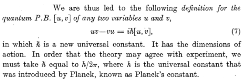
The notation for the reduced Planck constant (1) is due to:
- Paul Dirac, The Principles of Quantum Mechanics, International series of monographs on physics, Oxford University Press (1930) [ISBN:9780198520115]
but Dirac did not stick to this notation in his publications, until:
- Paul A. M. Dirac, p. 208 in: Théorie du Positron, Proceedings of Structure et propriétés des noyaux atomiques, Solvay Conference (1933) 203-212 [full:pdf]
Further discussion may be found in any monograph on quantum mechanics (see references there).
See also:
-
Simon Donaldson, Planck’s constant in complex and almost-complex geometry, XIIIth International Congress on Mathematical Physics (London,
2000), 63–72, Int. Press, Boston, MA, 2001
-
Wikipedia, Planck’s constant
Last revised on December 7, 2023 at 15:15:45. See the history of this page for a list of all contributions to it.